Overview of Data Flow Analysis
我们关心的就是 how data flows through CFG?
具体地,是 how
- application specific data
flows through
- nodes (i.e. basic blocks) and
- edges (i.e. control flow)
of the CFG (i.e. the program)
绝大多数分析,都是 over-approximation: what you output may be true, and if it's true, you should (nearly) always output.
- 又称为 may analysis
但是,还有一种分析,是 under-approximation: what you output must be true, and you don't have to output all true information.
- 又称为 must analysis
两者 analysis,都是为了保证结果在一定层面上的可靠性。
例子
对于符号分析:
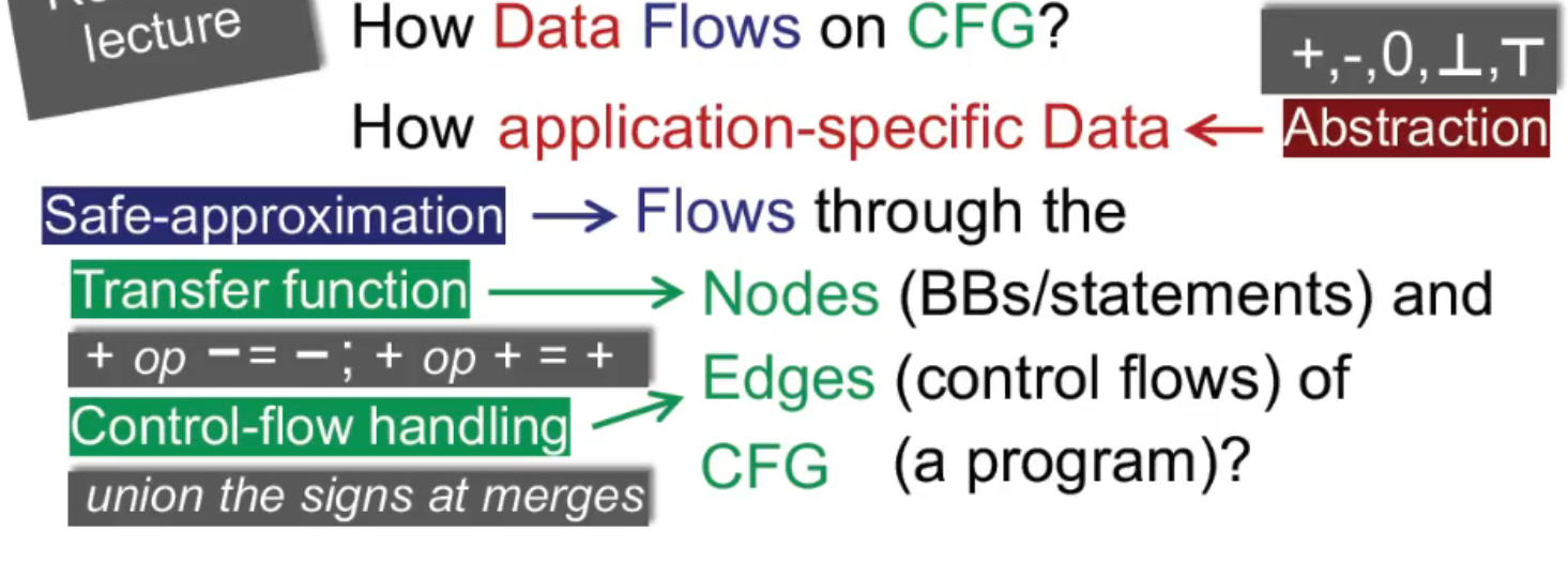
因此,不同的 data flow analysis 有
- different data abstraction
- and different flow safe-approximation strategies,
- i.e.,different transfer functions and control-flow handlings
Preliminaries of Data Flow Analysis
Input and Output States
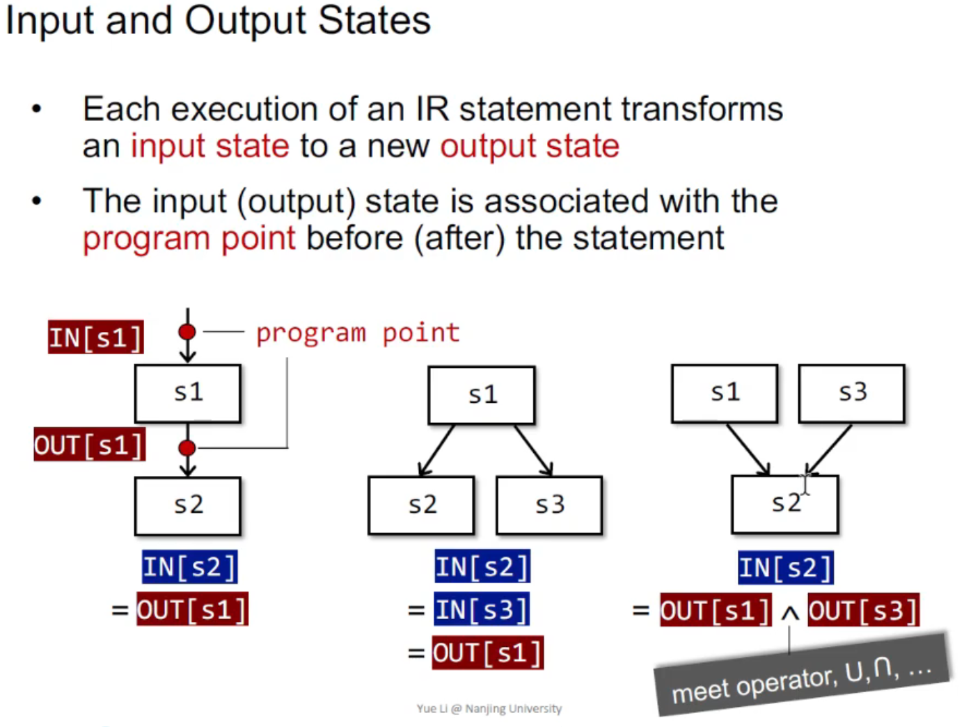
总结:我们进行 data flow analysis 的目的是,对于每一个红点(program point),我们需要 associate it with a data-flow value that represents an abstraction of the set of all possible program states that can be observed at that point.
Notation for Control Flow Constraints
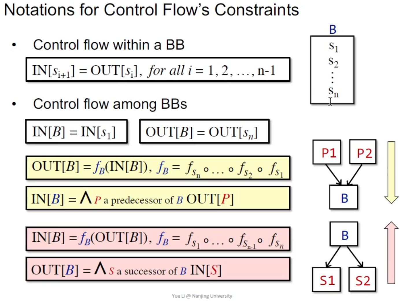
如图,黄色的是 forward analysis,红色的是 backward analysis。
- Program point 是值
- statements 是转移函数
- basic block 是多个转移函数的复合(也是一个转移函数)
- basic blocks 之间传递信息的时候,需要用到 \(\bigwedge\) 符号进行聚合
总结:我们进行 data flow analysis 的方法是,find a solution to a set of safe-approximation-directed constraints on the IN[s]'s and OUT[s]'s,for all statements s.
- constraints based on semantics of statements (transfer functions)
- constraints based on the flows of control
Reaching Definitions Analysis
定义:A definition d at program point p reaches a point q if there is a path from p to q such that d is not "killed" along that path
也就是说:我在 p 处刚定义了 d,如果有一条路径能从 p 到 q,而且其中 d 没有被重新定义,那么,就说 d 可以 reach p。
- 由于有路径 ≠ 程序实际上会走那条路径,reaching analysis 其实是 may analysis
例子 1
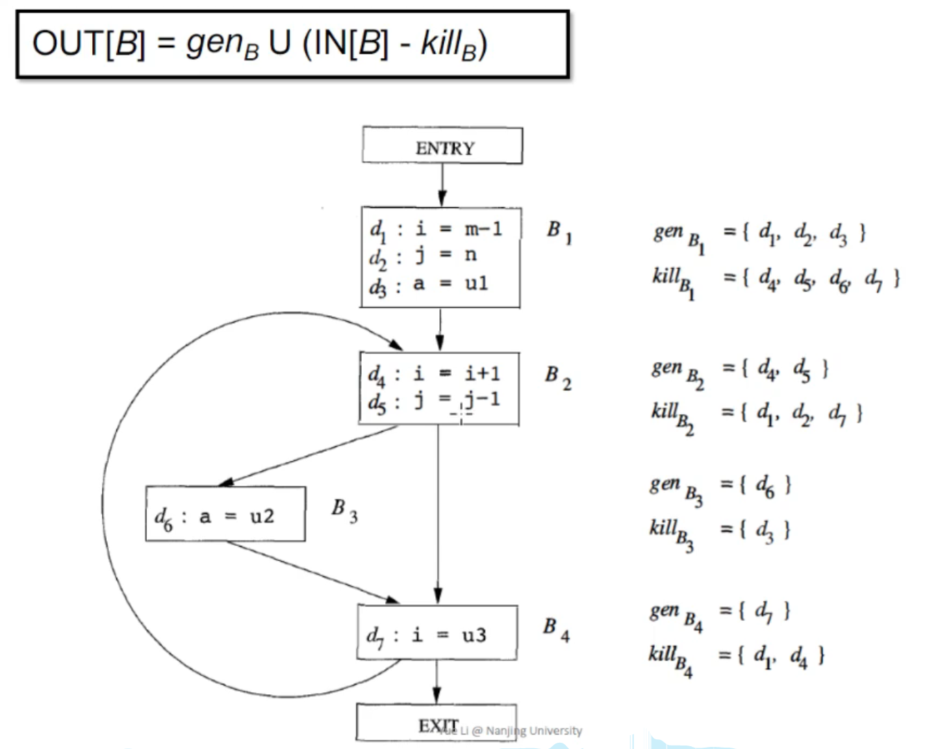
如图,对于 B1,由于 d1: i, d2: j, d3: a,因此,
- d1 -> i -> kills d4, d7
- d2 -> j -> kills d5
- d3 -> a -> kills d6
从而:\(kill_B = \set {d_4, d_5, d_6, d_7}\)
下面,我们给出一个完整的定义:
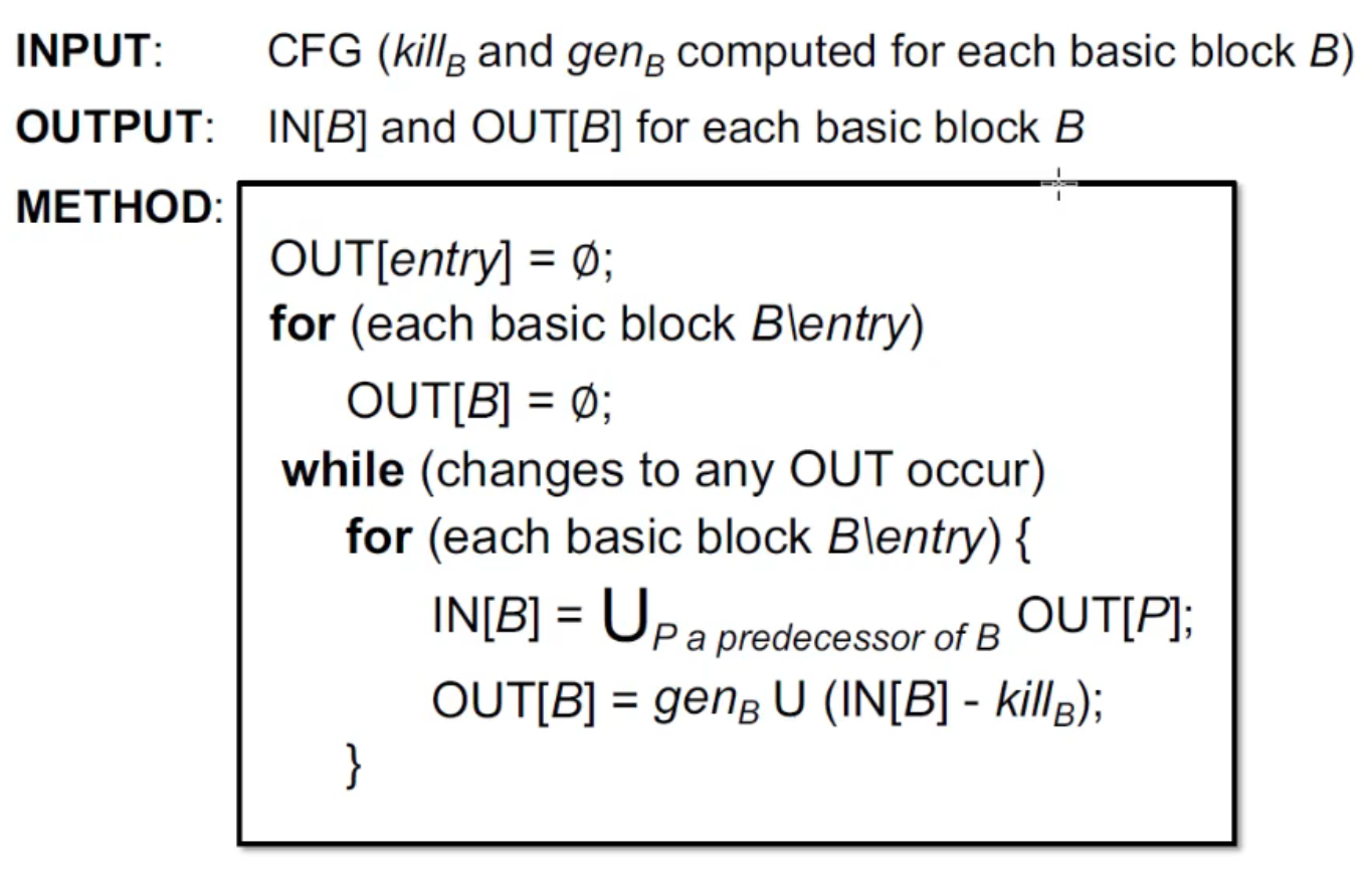
- Transfer function:\(OUT[B] = gen_B \bigcup (IN[B] - kill_B)\)
- Control flow: \(IN[B] = \bigcup_{P\text{ a predecessor of }B} OUT[P]\)
- We use over-approximation as safety requirement here
从而,算法如下:
例子 2
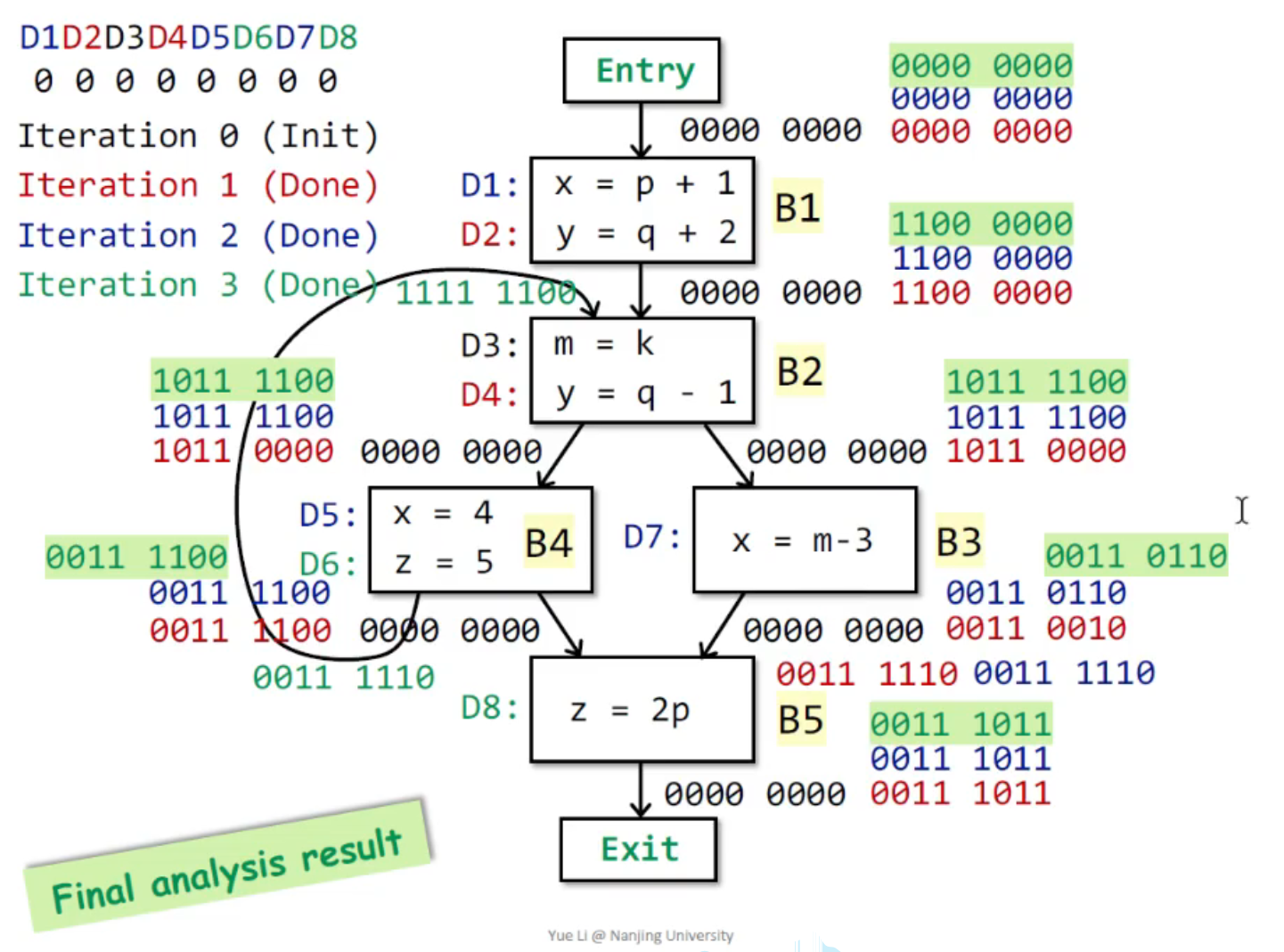
Why this iterative algorithm can finally stop?
我们令 \(B_n(x)\) 为 \(B_n\) 在第 X 轮时的输出。
不难发现:\(B_n(x)\) 只和 \(B_{n}(x-1), B_{n+1}(x-1), \dots, B_{N}(x-1), B_1(x), B_2(x), \dots, B_{n-1}(x)\) 有关。
从而,严格地说,如果 \(\forall n \geq n_0: B_n(x-1) \subseteq B_n(x) \land \forall n < n_0: B_n(x) \subseteq B_n(x+1)\),那么:\(B_{n_0}(x) \subseteq B_{n_0}(x+1)\)。
通过数学归纳法,我们不难证明:\(\forall n, x: B_{n}(x) \subseteq B_{n}(x+1)\)。
因此,如果有 changes to any OUTPUT occur,则必然递增前是递增后的严格子集,也就是 \(B_n\) 呈单调增加。
由于集合最大只能是所有 \(B_n\) 全满,因此,迭代的次数必然小于 \(N * \# \text{ of definitions}\)。从而,一定可以 stop。
Why we end when OUT stay that same?
如果 OUT stay the same,就会有 \(B_{n}(1, \dots, n) = B_{n-1}(1, \dots, n)\)。
从而,下一轮中,
- \(B_{n+1}(1) = f(B_n(1, \dots, n)) = f(B_{n-1}(1, \dots, n)) = B_{n}(1)\)
- 根据 (1):\(B_{n+1}(2) = f(B_{n+1}(1), B_n(2, \dots, n)) = f(B_{n+1}(1),B_{n-1}(2, \dots, n)) = B_{n}(1)\)
- 根据 (1), (2):\(B_{n+1}(3) = f(B_{n+1}(1,2), B_n(3, \dots, n)) = f(B_{n+1}(1,2),B_{n-1}(3, \dots, n)) = B_{n}(3)\)
- \(\dots\)
如此归纳,从而,\(n+1\) 轮中,所有的 \(B_{n+1}(x)\) 也都等于 \(B_n(x)\)。我们无需再迭代下去了。