Recap
What we learnt in the previous course:

- More layers, more fitting power
- But, linear * linear = still linear, non-linear * non-linear = "more" non-linear
- And it is ReLU that makes each layer non-linear
What we shall learn in this course:

- Convolution: extract the 2D structure without information loss
- Pooling: down-sampling that preserves the 2D structure
- Normalization: prevent over-fitting
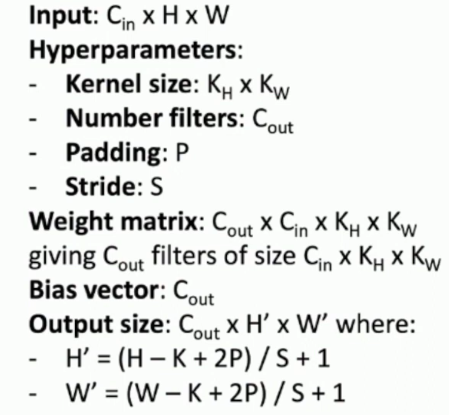
Convolution Layers
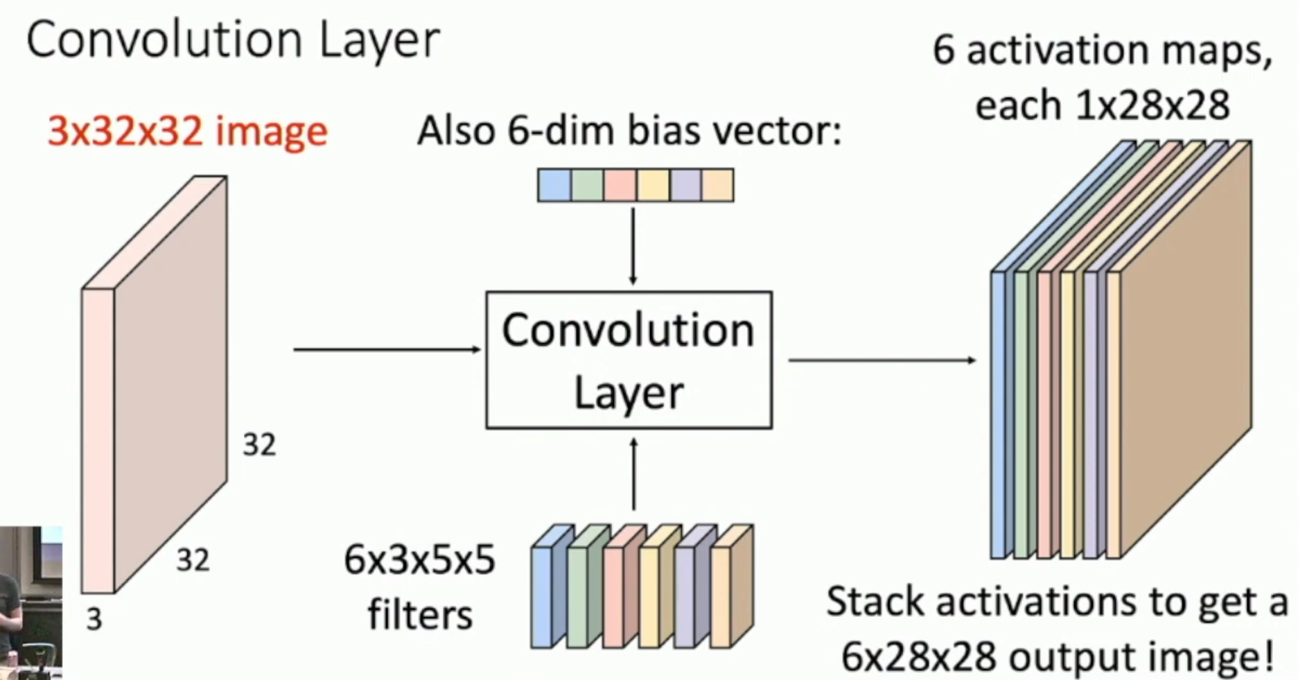
图片尺寸:每个像素的信息量 × 像素行数 × 像素列数
卷积核尺寸:希望生成的 activation map 的数量 × 每个像素的信息量 × 卷积核行数 × 卷积核列数
卷积过程:
- 将一个卷积核(i.e. 对应着“每个像素的信息量 × 卷积核行数 × 卷积核列数”)施加于“每个像素的信息量 × 像素行数 × 像素列数”上,(然后再加上一个 bias),从而得到“卷积后行数 × 卷积后列数”
- 对每一个卷积核都这样处理,从而得到“希望生成的 activation map 的数量 × 卷积后行数 × 卷积后列数”
实际意义:
- “6”:每一个希望每一个 bias vector 能够 extract different features
- “3 × 5 × 5”:每一个 bias vector 都是 2D 的(如上图,是 3 × 5 × 5 的带有深度的 2D 卷积核,而非 75),非常适用于图片
- “6 × 3 × 5 × 5”:bias vector 的参数比全连接层少得多,从而反向梯度传播的计算量大大减小
注意:上图的左侧只是一张图片的情况。实际上,我们需要很多 batches(下面记为 N)。因此,实际的运算过程如下图:
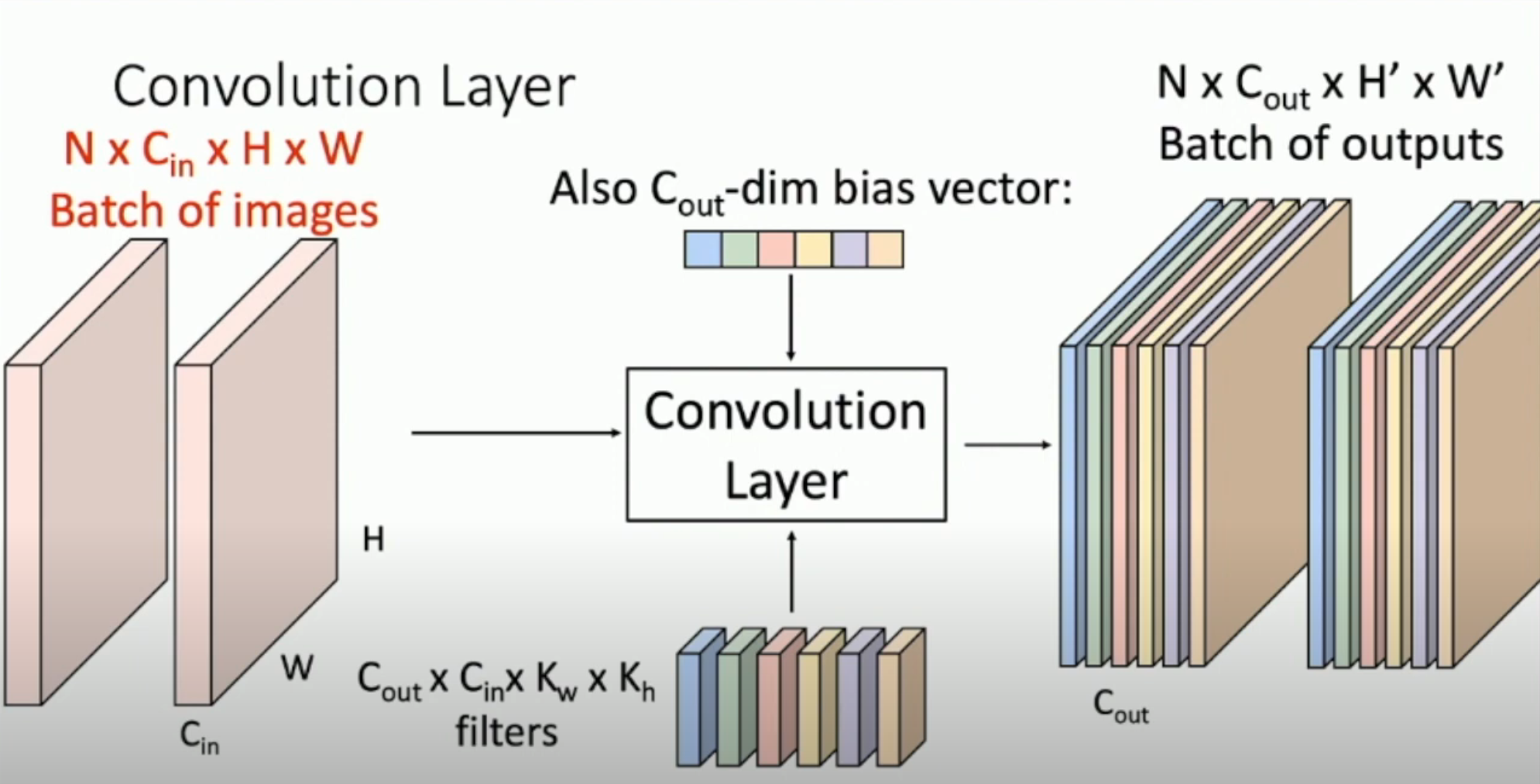
Stacking Convolutions
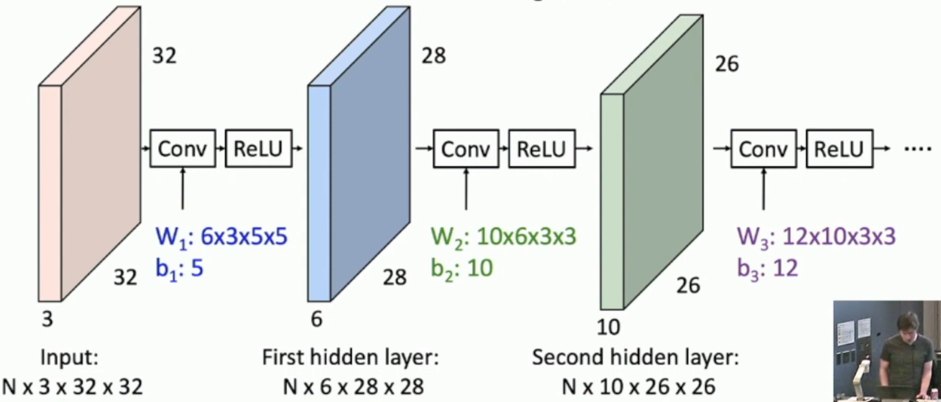
- Typo: b1 should be 6, not 5
由于卷积和卷积的复合还是卷积,因此,我们需要像应对神经网络的线性性一样,为每一层的结果施加 ReLU 算子。
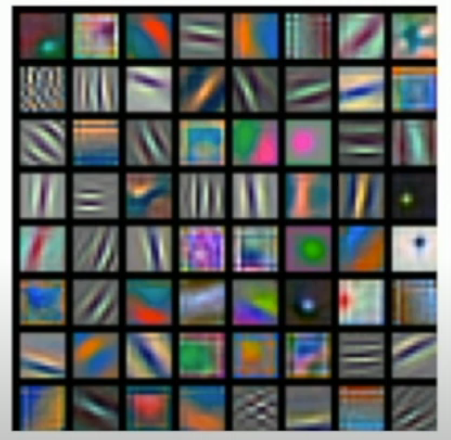
What do convolutional filters learn?
First-layer conv filters: local image templates (often learns oriented edges, opposing colors)
Receptive Fields
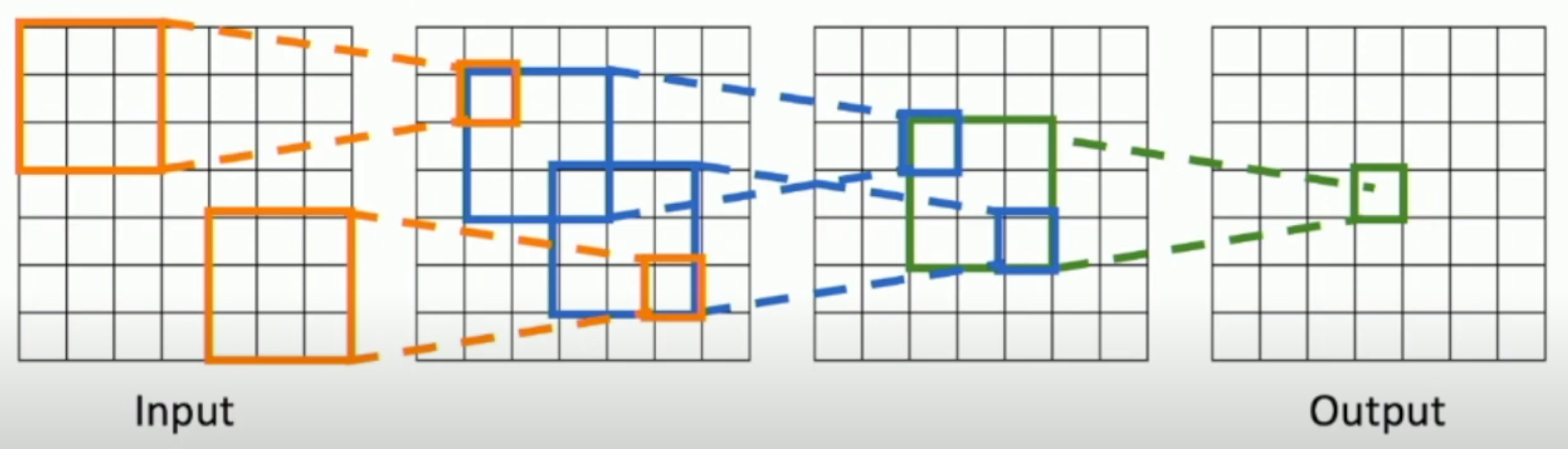
The receptive field (of some pixel in the output) in some layer is the group of pixels in that layer which can affect the pixel in the output layer.
For example,
- The receptive field in the previous layer is the area surrounded by green lines
- The receptive field in the input is the entire input
As you can see, with a \(k\)-by-\(k\) convolution kernel, we can expand the edge length of the receptive field by \((k-2)\) for each layer.
However, it's way too slow due to its linear growth.
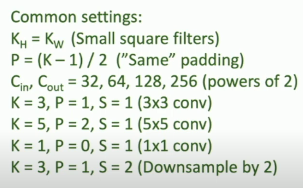
Acceleration
We can use convolution with stride ≥ 2.
Summary & Practices
Recap:
- Filter size determines the receptive fields
- Number of filters (also bias vector) determines the features you want to extract
- Stride determines how much you want to down-sample
- Actually, "down-sampling" in CNN is usually done by both convolution layer with stride ≥ 2 and pooling layer
Pooling Layer
Pooling layer is a way to
- down-sample
- introduce invariance to small spatial shifts
本质上,pooling layer 就是一个 fixed down-sampling method.
Pooling layer 只有两个超参数:K 和 S。意义同 convolution layer。
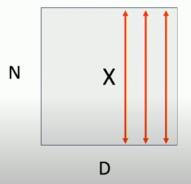
Batch Normalization
我们对 batch 里面的 \(N \times D\)(\(N\) 是 batch size,\(D\) 是向量的维数)矩阵,每一列进行这样的 normalization。也就是说,对于长度为 \(D\) 的向量的每一个 element,我们 batch 里都有 \(N\) 个,因此我们求出这 \(N\) 个数的方差和平均值,然后进行处理(如下图,我们一条条红线进行处理)
原因:
- 论文原话:Helps reduce "internal covariate shift", improves optimization
- 我们可以认为:保持分布的一阶、二阶矩不变,并且防止梯度爆炸/消失
方法: $$ \widehat x^{(k)} = \frac {x^{(k)} - \mathrm E[x^{(k)}]} {\sqrt{\mathrm{Var}[x^{(k)}]}} $$
- 注意:实际中,为了保证数值稳定,我们需要在分母的根号里加上一个 \(\varepsilon\)。
工程实践:
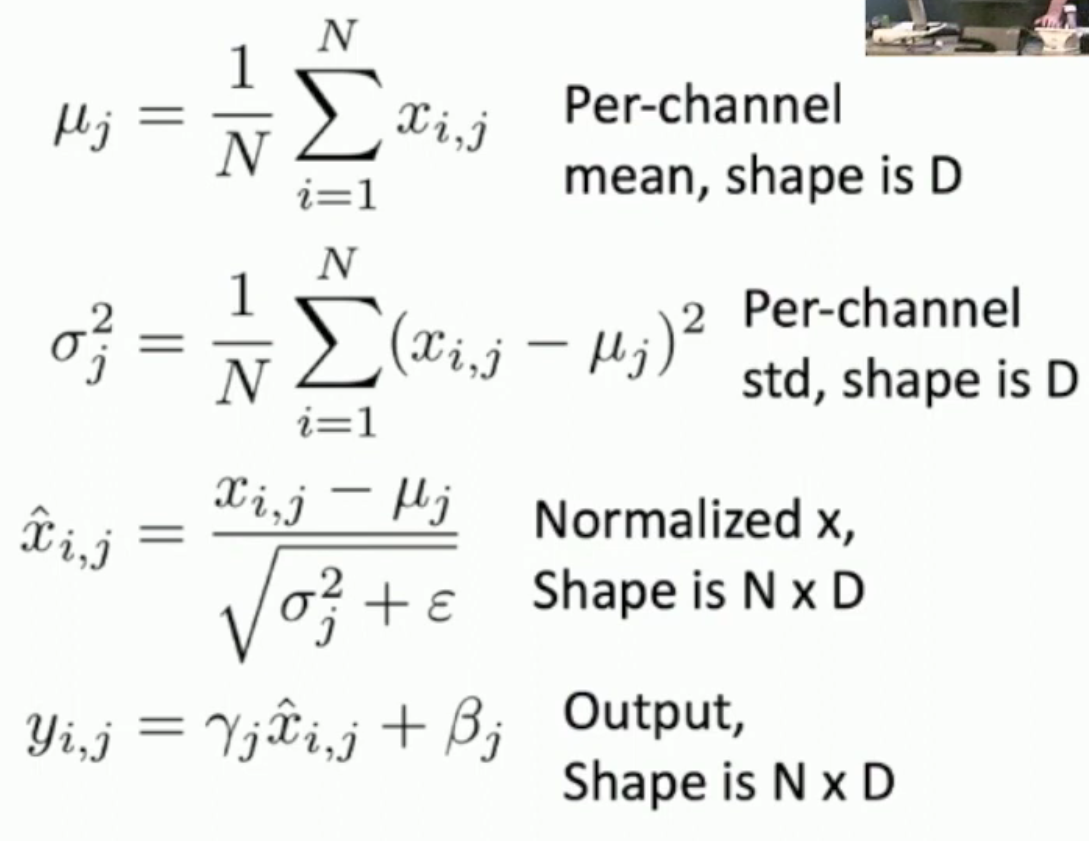
如图,我们还会加入 \(\gamma, \beta\) 这两个 learnable parameters 来使得模型还有调整自己的“余地”(提升模型的 power,避免欠拟合)。
Test-Time
Batch normalization 要求我们在训练的时候,必须一次输入 \(N\) 个向量。但是,在 test 的时候,一次只有一个输入。
因此,我们会将 μ 和 σ 设置成训练时的平均值:

同时,由于 μ, σ 变成常量之后,就是线性变换,因此,我们可以将 normalization 和 γ, β 二合一。
进一步,我们可以把这个线性变换和之前的卷积层/全连接层(注意卷积也是线性变换)再次二合一,从而实现 zero computational overhead at test-time。
Batch Normalization For ConvNets
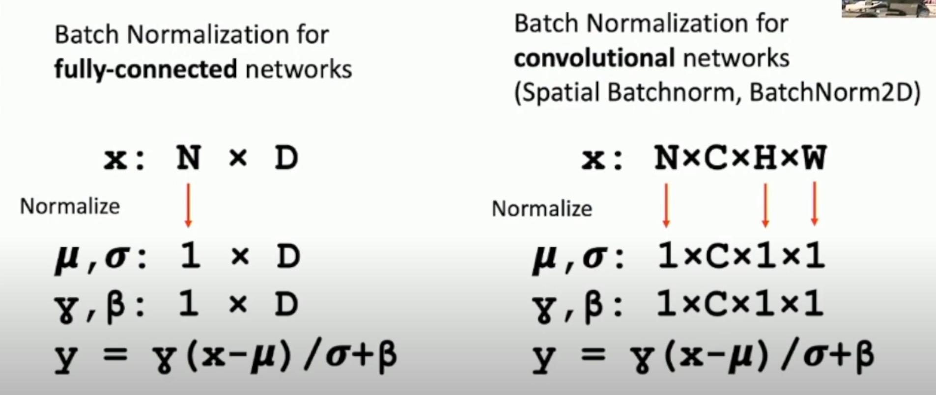
注意:对于图片而言,我们把每张图片的每一个像素视为 batch 里的一份,也就是说,batch 的大小为 N × H × W(伪代码: normalize(NCHW, dim=[0,2,3])。
Cons and More
Batch Normalization 虽然可以大大提升收敛速度,但是
- 理论上没有什么保障
- 实际应用中,由于训练和测试的网络是不一样的,因此容易出 bug

就第二个问题,后来又有 layer norm (e.g. transformer), instance norm, group norm 被使用。这三种方法不需要 batch,因此训练和测试的网络是一样的。如下图所示:
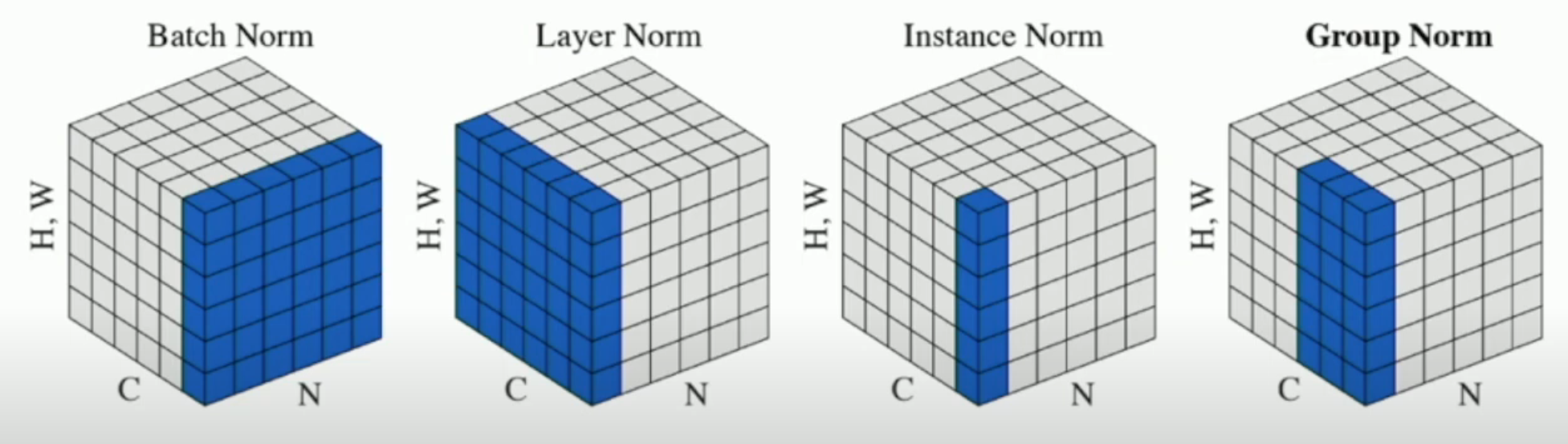
其中,
- batch norm 就是所有图像的一个通道
- layer norm 就是一个图像的所有通道
- instance norm 就是一个图像的一个通道
- group norm 就是一个图像的多个通道