5. Neural Networks
Feature Extraction
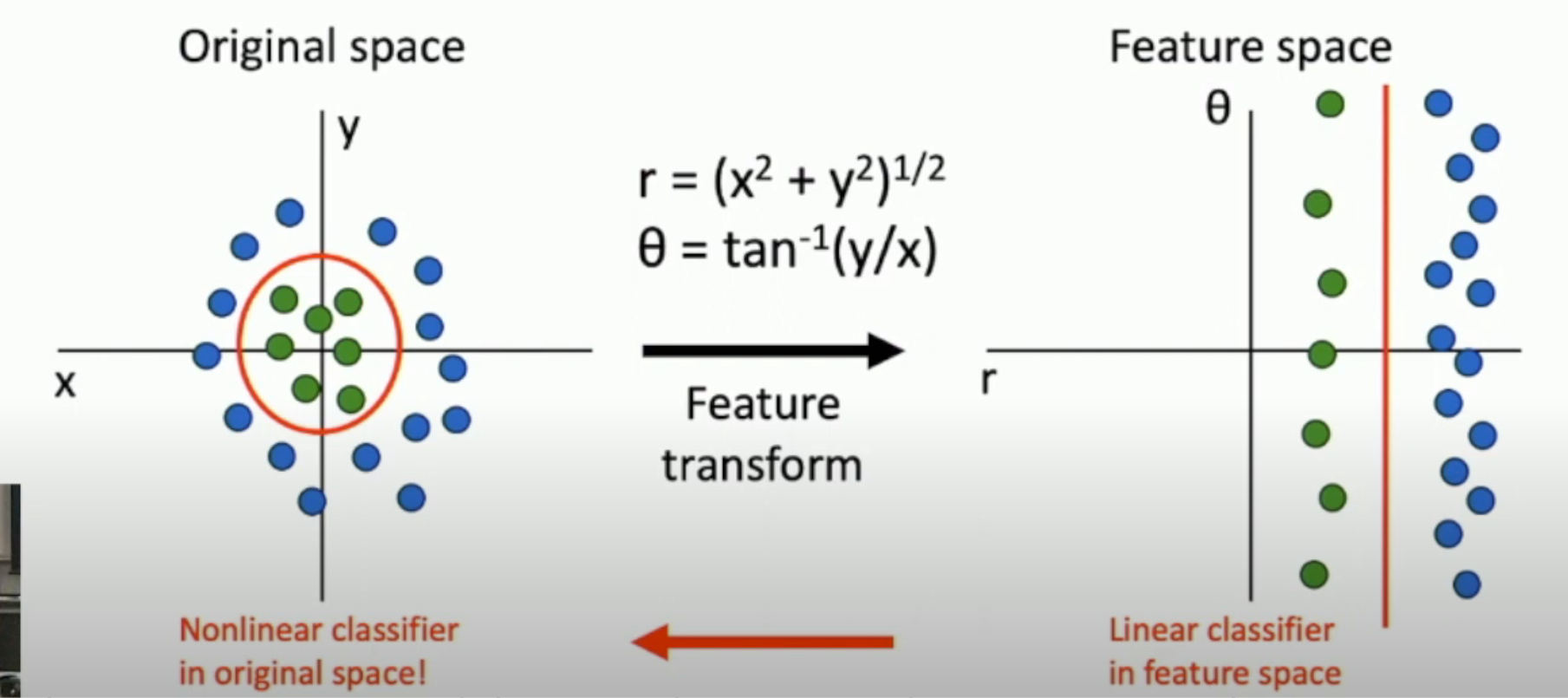
Raw data sometimes hardly mean anything, so in order to extract the implicit features, you have to map it to feature space, like this image below:
Color Diagram
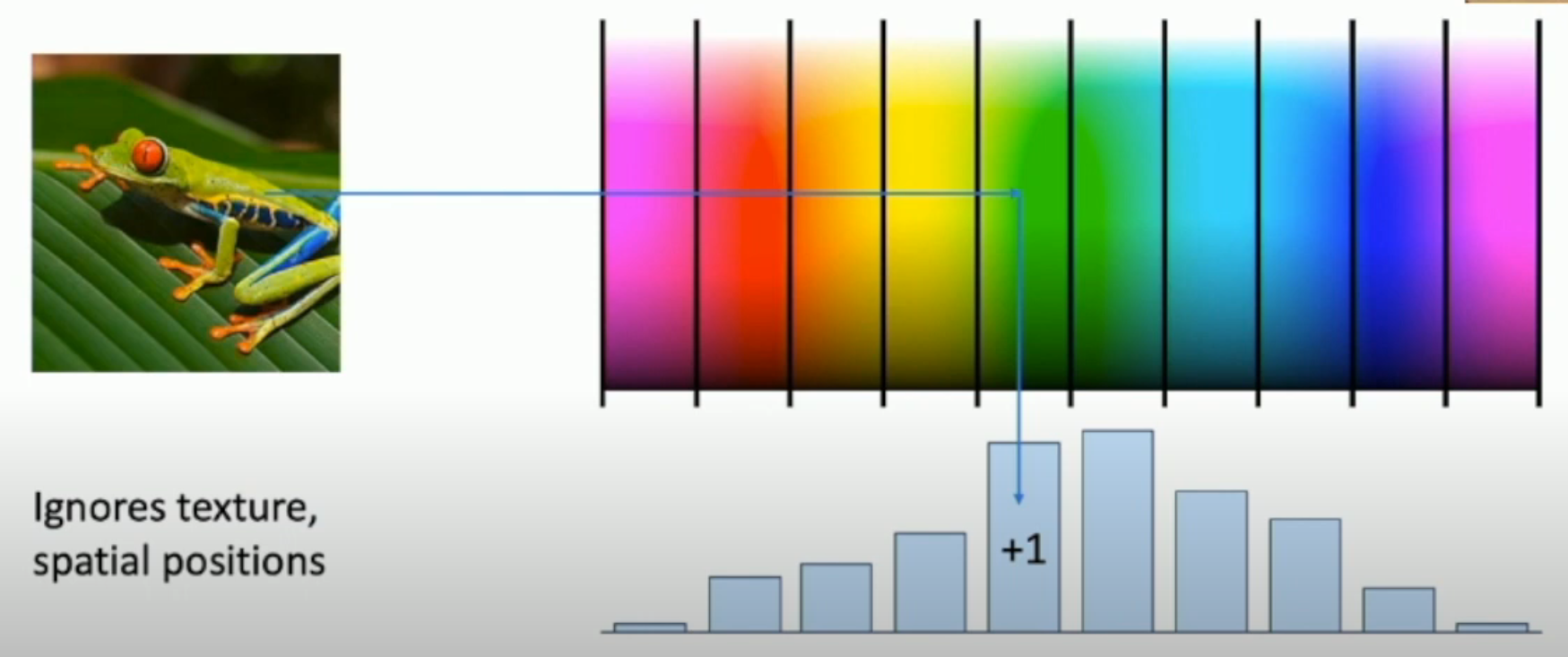
As shown in the image, only the color feature is extracted, and the position feature is discarded. Thus, this extraction algorithm is robust with object shift and rotations.
Histogram of Oriented Gradients
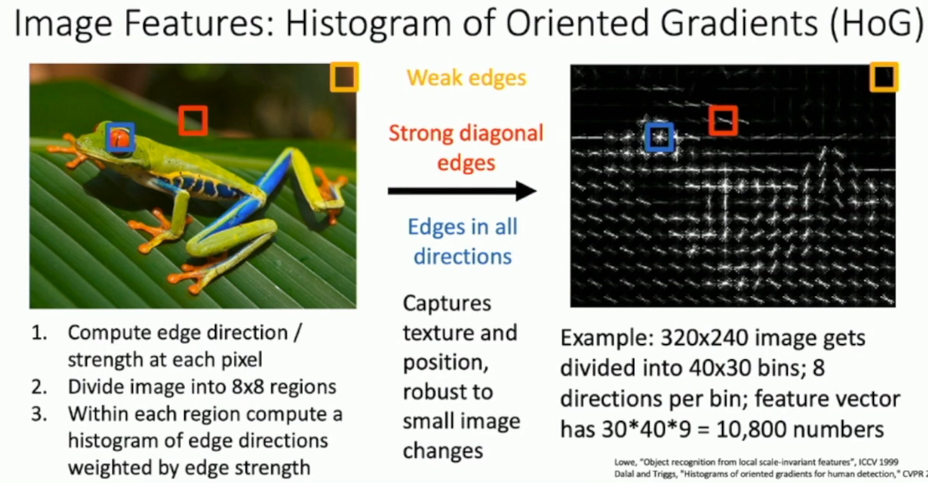
As opposed to "color diagram", the color feature is discarded, and what remains is the gradient of the light.
Bag of Words
In the two cases above, we have to manually specify the feature that we want to extract. But the "bag of words" algorithm can somehow "learn" from data what features to extract.
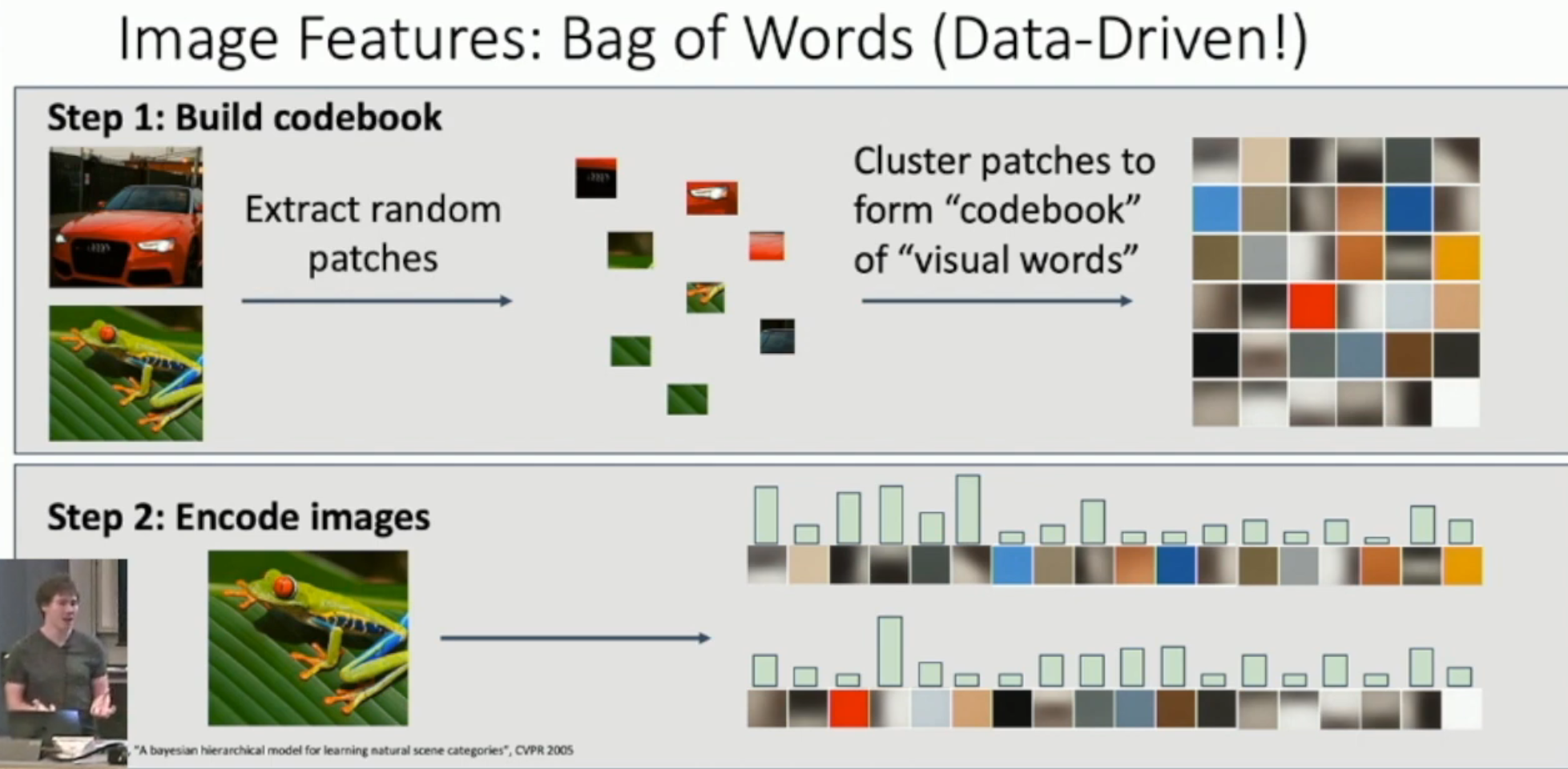
如图:
- 首先从图片中抽取出 random patches(patch 就是从图像中“切下”的一小块。我们认为一个 patch 里面就已经含有了一定的局部特征)
- 我们将 patches 进行聚类,将每个聚类的中心映射到 one-hot encoding 的一个向量
- 之后,我们把每一个 test image 的每一个 patch,通过 codebook,找到距离最近的聚类中心对应的 one-hot vector。然后将所有这些 one-hot vector 相加,得到这个图像的 vector。
Traditional Feature Extraction and DNN

This traditional pipeline consists of basically two components:
- feature extraction module, which is untunable
- learnable module, which you can tune
However, we also want to tune the feature extraction module. And that's why we use DNN:
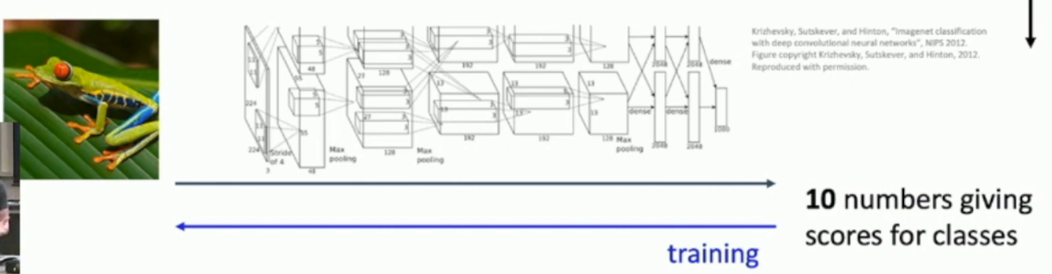
As you can see, we can tune both the feature extraction module and the learnable module during training.
Geometric View of Neural Network
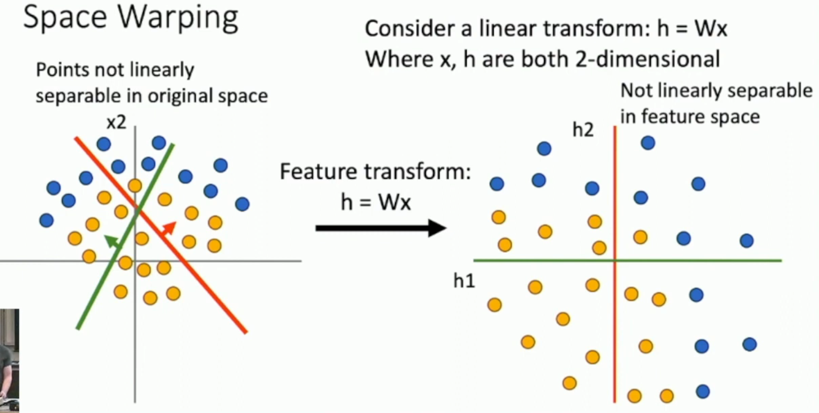
Without activation function, the neural network is just layers and layers of affine transformation, useless!
Just like the image below, no matter how many time you apply affine transformation, the data is still linear inseparable!
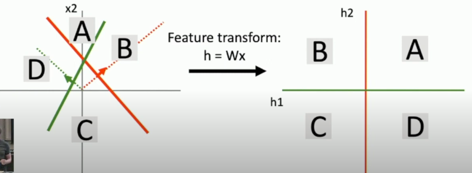
But, with ReLU,
- B will be compressed to red axis (since B corresponds to the negative area of green feature)
- D will be compressed to green axis (since C corresponds to the negative area of red feature)
- C will be compressed to the origin point
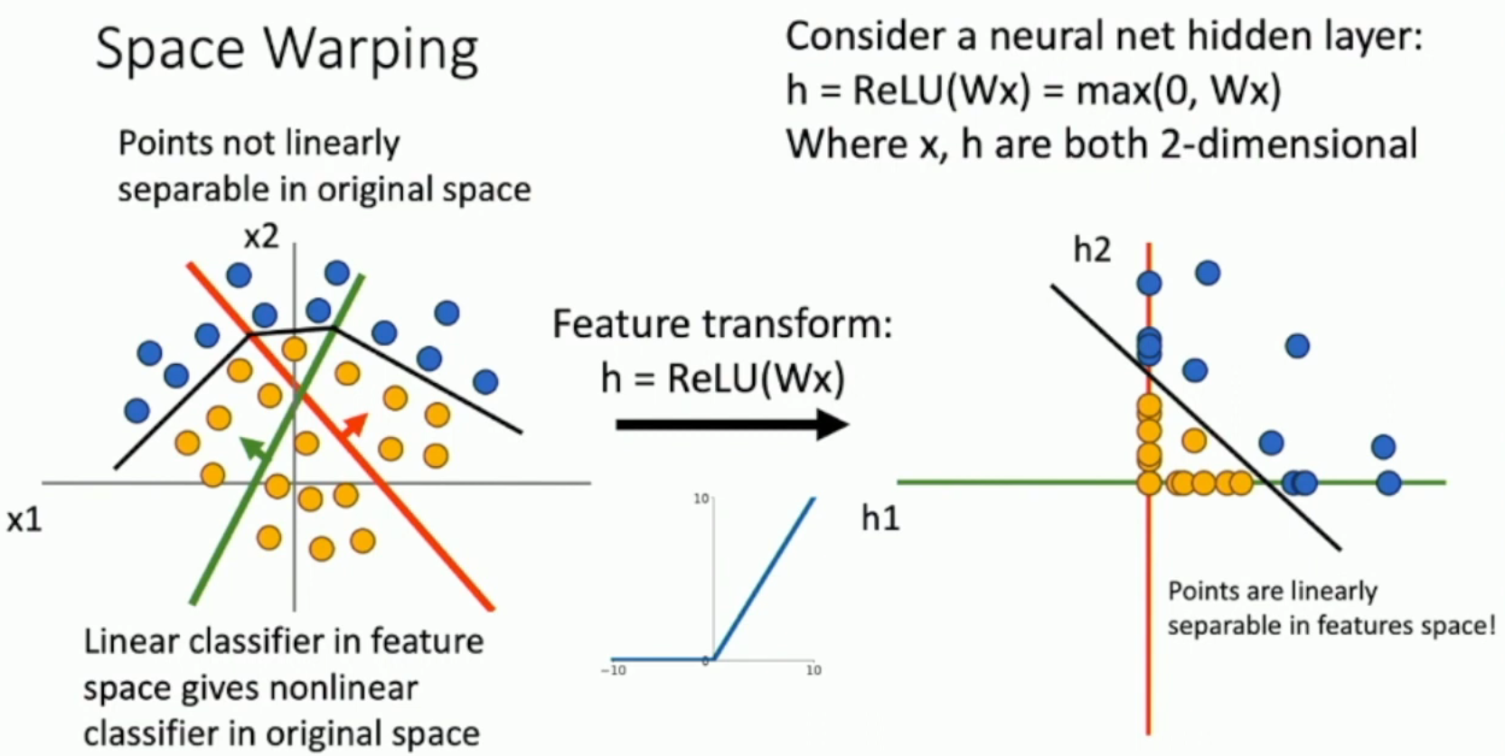
Now its linear separable, and the boundary is non-linear.
Universal Approximation Property
对于 ReLU,我们可以通过 bump function(可以由四个 ReLU 相加而成)来拟合任何函数。
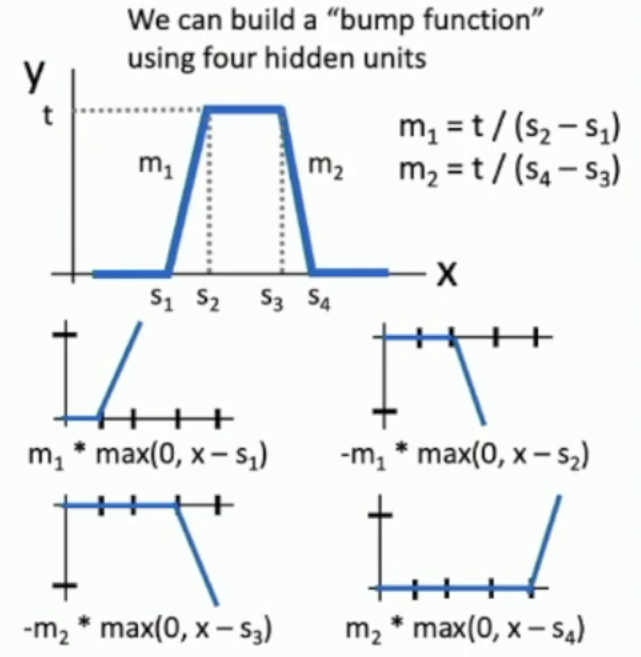
- 不过,在实际的训练中,神经网络并不用的 bump function 来进行拟合,而是通过调整其它的参数
Back Propagation
前馈神经网络中,主要由三个参数(不用纠结下面具体的编号,like 从 0 开始还是从 1 开始,只需知道大致情况即可):
- \(w_{i, j}^{(k)}\):第 k 层从 i 连到 j 的权重
- \(z_j^{(k)}\):第 k 层第 j 个神经元的聚合
- \(a_i^{(k)}\):第 k 层第 i 个神经元的输出
- 从聚合到输出,经历了一个 ReLU 函数
从而:
其中,我们传播时要记录的就是 \(\par C a, \par C w\)。
由于我们用的是 ReLU 激活函数,故 \(\par a z\) 很简单,i.e. \(\par a z := \par {\operatorname*{ReLU}(z)}{z} := \text{if z > 0 then 1 else 0}\)
\(\par z {w \text{ or }x}\) 也很简单,i.e. \(z:=\sum w \cdot x \implies \par z {w \text{ or }x} := x \text{ or }w\)