Recap: Gaussian Elimination

高斯消元法，就是：

如果第 \(n\) 行第 \(m\) 列不为 0，就逐一去减下面的行，然后再处理第 \(n+1\) 行第 \(m+1\) 列
如果第 \(n\) 行第 \(m\) 列为 0，就试图和下面的某一个为 0 的行进行交换，然后再进行第一步
如果第 \(n\sim N\) 行第 \(m\) 列均为 0，那么就不管这一列了，处理第 \(n\) 行第 \(m+1\) 列去

处理完毕之后，从下往上 back substitution。

如果某一行全零，如果右侧也为 0，那就是自由变量
如果某一行全零，右侧不为 0，那就方程无解

Better Gaussian Elimination: Pivoting Strategy

Problem: Small pivot elements may cause trouble.

原因： - 如果 pivot 过小，那么，为了消去下面的行，我们就需要乘以一个很大的 factor，导致本行的其他数过大，从而导致本行与下面的行相加之后，rounding 的时候产生很大的的绝对误差。

比如说：

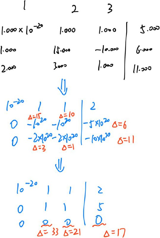
其中，\(\Delta\) 指的是误差范围。

Partial Pivoting

每一次，我们都选取该列、待计算行以下的最大的 pivot 作为目标行，和本行进行交换。

额外操作的时间复杂度是：\(\mathcal O(\sum_i^n (n-i)^2) = \mathcal O(n^2)\)。其中，需要 \(\mathcal O(n^2)\) 的比较。

Scaled Partial Pivoting

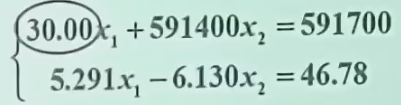
对于如上的算式，如果我们还是选取最大的 pivot 进行计算，那么就会导致：

30.00 591400    591700
5.291 -6.130    46.78

30.00 591400    591700
0    -104300   -104400

Result: 
x2 = 1.001
x1 = -9.713

虽然 5.291 / 30.00 不大，但是乘以 591400 后，就会变得巨大。

因此，我们需要将每一行 scale 一下：一行中的所有数除以该行的最大（绝对）值。然后，我们再通过 partial pivoting 进行比较。

也就是说：

30.00 591400    591700 // 5.043e-5  1 
5.291 -6.130    46.78  // 0.8631    1

5.291 -6.130    46.78  // 0.8631    1
30.00 591400    591700 // 5.043e-5  1 

5.291 -6.130    46.78 
0     591400    591400

Result: 
x2 = 1.000
x1 = 10.00

这样就对了。

注意：Scaled Partial Pivoting 需要提前计算好每一行的最大值。并且之后即使发生了变化，也还是沿用这个最大值。

额外操作的时间复杂度是：\(\mathcal O(n^2 + \sum_i^n (n-i)^2) = \mathcal O(n^2)\)。其中，需要 \(\mathcal O(n^2)\) 的比较和浮点除法。
否则，额外的时间复杂度就是：\(\mathcal O(\sum_{i}^{n}(n-i)^2) = \mathcal O(n^3)\)。其中，需要 \(\mathcal O(n^2)\) 的浮点除法和 \(\mathcal O(n^3)\) 的比较。

Complete Pivoting

简单来说：我们不仅换行，还换列。

1     2
30.00 591400    591700
5.291 -6.130    46.78

2      1
591400 30.00    591700
-6.130 5.291    46.78

2      1
591400 30.00    591700
0      5.291    52.92

2      1
1      0        1.000
0      1        10.00

Result: 
x2 = 1.000
x1 = 10.00

如果我们能够把最大的数换到 pivot，那么，任何其他加减操作，其加减的大小都不会超过这个最大的数。

额外的时间复杂度就是：\(\mathcal O(\sum_{i}^{n}(n-i)^2) = \mathcal O(n^3)\)。其中，需要 \(\mathcal O(n^3)\) 的比较。

总结

Partial pivoting 是最快的方法，因为不涉及浮点除法（常数很大）。Scaled partial pivoting 也还好。

但是，complete pivoting 虽然不会增加 Gaussian Elimination 的渐进复杂度，但是会造成以下后果：

There is an apparent misunderstanding of how pivoting is used in the LU factorization. It is not used to permute the original matrix before the actual elimination algorithm, but instead to choose pivots by permuting the "intermediate" partially eliminated matrices generated during the individual steps of the elimination.

A step of an LU factorization can be expressed as \(A_k = L_k'A_{k-1}\), where \(A_0:=A\) and \(L_k'\) is an elementary unit lower triangular matrix introducing zeros below the diagonal of the \(k\)-th column of \(A_{k-1}\), eventually meaning that \(A_n:=U\) is upper triangular.

The partial pivoting introduces permutation matrices \(P_k\) such that the \((k,k)\) entry of the row-permuted matrix \(P_k A_{k-1}\) is the largest in magnitude compared to the other entries in the same column below the diagonal of \(A_{k-1}\). In complete pivoting there is an extra permutation matrix \(Q_k\) which together with \(P_k\) selects the pivot by both row and column permutation \(P_k A_{k-1} Q_k\) such that the largest element in magnitude of the trailing uneliminated part is brought to the current pivoting entry. If I remember correctly, the Rook's pivoting strategy is similar to the complete pivoting in terms of utilization of both row and column permutations.

In any case, \(PAQ=LU\) is how the results of all considered pivoting techniques could be related to the original matrix \(A\) and the resulting triangular factors, where \(P\) and \(Q\) are permutations (\(Q=I\) for the partial pivoting). However, the sequence of elementary permutations forming both \(P\) and \(Q\) depends on the intermediate values appearing in the partially reduced matrices \(A_k\), not on the values in the original matrix \(A\) itself.

因此，很多时候，还是不用 complete pivoting 为好。

LU 分解

如果我们不进行任何的行交换，对一个矩阵进行上对角化，那么，我们对一个 \(I\) 施以对应的变换，就可以实现 \(I\) 变成下对角阵。

i.e. \(L_n \dots L_2 L_1 A = U \implies A = (IL_1^{-1}\dots L_n^{-1}) U = LU\)

如果我们需要复用这个矩阵（比如说解很多次方程），我们可以先将矩阵 LU 分解（可以用 complete pivoting），就可以在之后的求解中，只需要 \(\mathcal O(n^2)\)。

每次求解时，只用计算 \(Ly=b\)，再计算 \(Ux=y\)。由于均为三角阵，因此无需消元，复杂度大大降低。

Special Type of Matrices

对于特殊矩阵而言，我们可以 take advantage of its properties，从而大大加速运算。

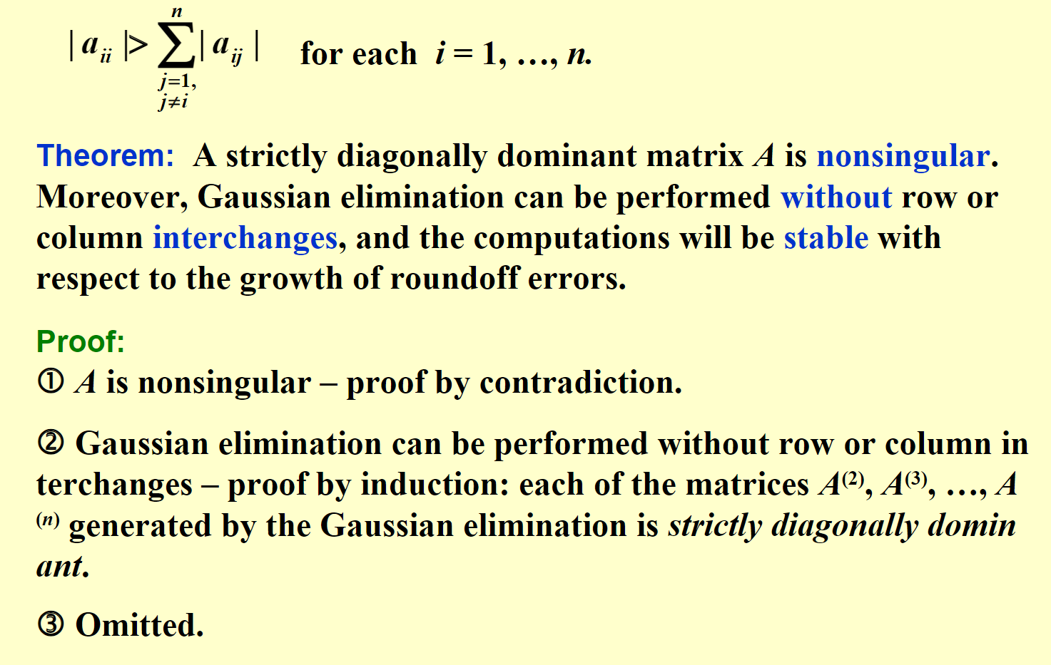
Strictly Diagonally Dominant Matrix

Choleski's Method for Positive Definite Matrices

如果 \(A\) 是正定矩阵，我们可以将其分解为 \(A = \widetilde L \widetilde L^t\)。这也被称为 LLT method（类似的还有 LDLT method）。

存在性证明：

首先，我们进行常规的 LU 分解。其中，我们希望 L 的对角线全为 1。

然后，将 U 分解成对角矩阵和对角线为 1 的矩阵。如图：

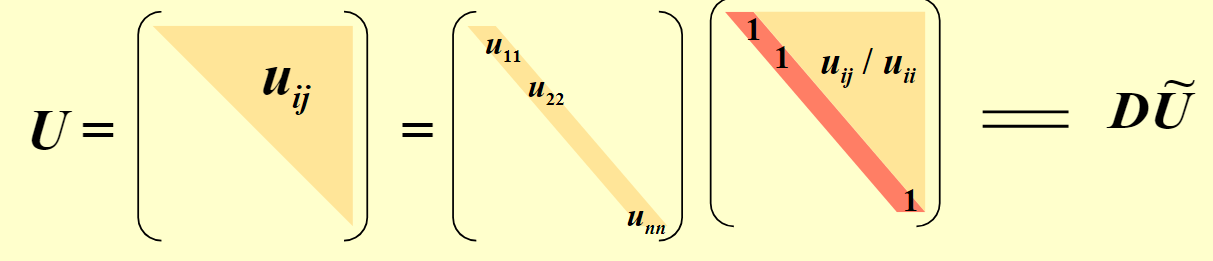
从而：\(LD\widetilde U = A = A^t = \widetilde U^t D L^t\)。由分解的唯一性：\(L = \widetilde U^t\)

从而：\(A = LDL^t\)。令 \(\widetilde L = LD^{1/2}\)，我们就可以得到我们希望得到的式子。

算法：

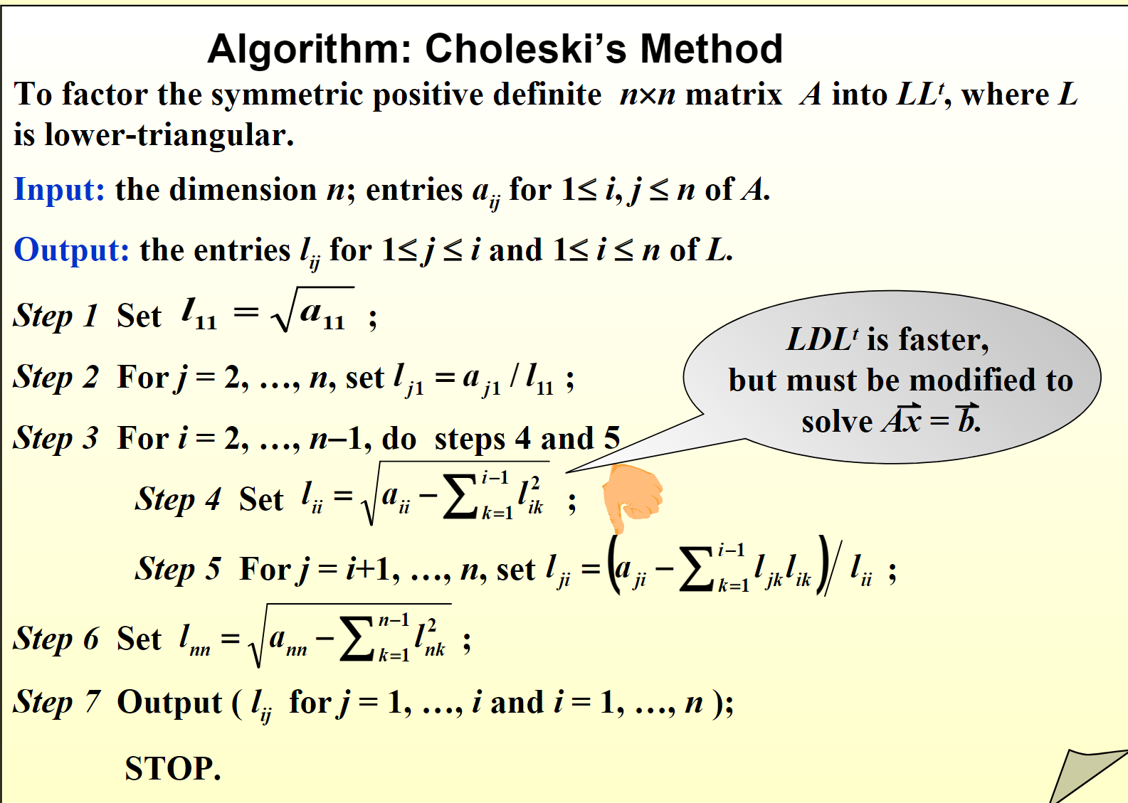
NOTE: Choleski's method 比一般的 LU 分解可以快上很多倍。因此，如果你的矩阵是正定的，就用 Choleski 的方法（i.e. LLT）求解吧。当然，也可以用 LDLT。不过前者更加 cache friendly。

Sidenote: LLT vs LDLT

LLT和LDLT都是矩阵分解的方法，用于解决线性方程组和矩阵求逆的问题。它们之间的主要区别在于对称正定矩阵的处理方式。

LLT分解：
LLT分解是对称正定矩阵的Cholesky分解的一种形式。
Cholesky分解是将对称正定矩阵分解为下三角矩阵和其转置的乘积的过程。即，如果 \( A \) 是对称正定矩阵，则存在一个下三角矩阵 \( L \)，使得 \( A = LL^T \)。
LLT分解的优点是计算相对简单，并且能够利用对称性节省计算量。
LDLT分解：
LDLT分解也是对称正定矩阵的分解方法，但它将矩阵分解为一个单位下三角矩阵、对角矩阵和其转置的乘积。即，如果 \( A \) 是对称正定矩阵，则存在一个单位下三角矩阵 \( L \) 和对角矩阵 \( D \)，使得 \( A = LDL^T \)，其中 \( D \) 的对角线元素是正的。
LDLT分解相比于Cholesky分解，具有更好的数值稳定性，在某些情况下可能更适合使用。

总的来说，LLT和LDLT分解都是用于解决对称正定矩阵的分解问题的方法，选择哪种方法取决于具体的应用场景和数值计算的需求。

三对角矩阵

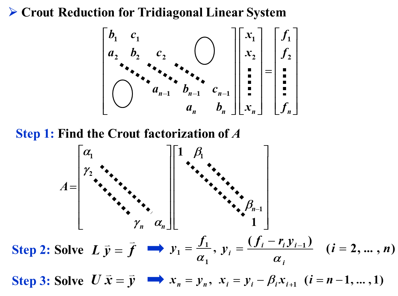
如上图，我们不需要使用 \(\mathcal O(n^2)\) 的方法来解决三对角矩阵，而是只需要采用 \(\mathcal O(n)\) 的递推进行计算即可。

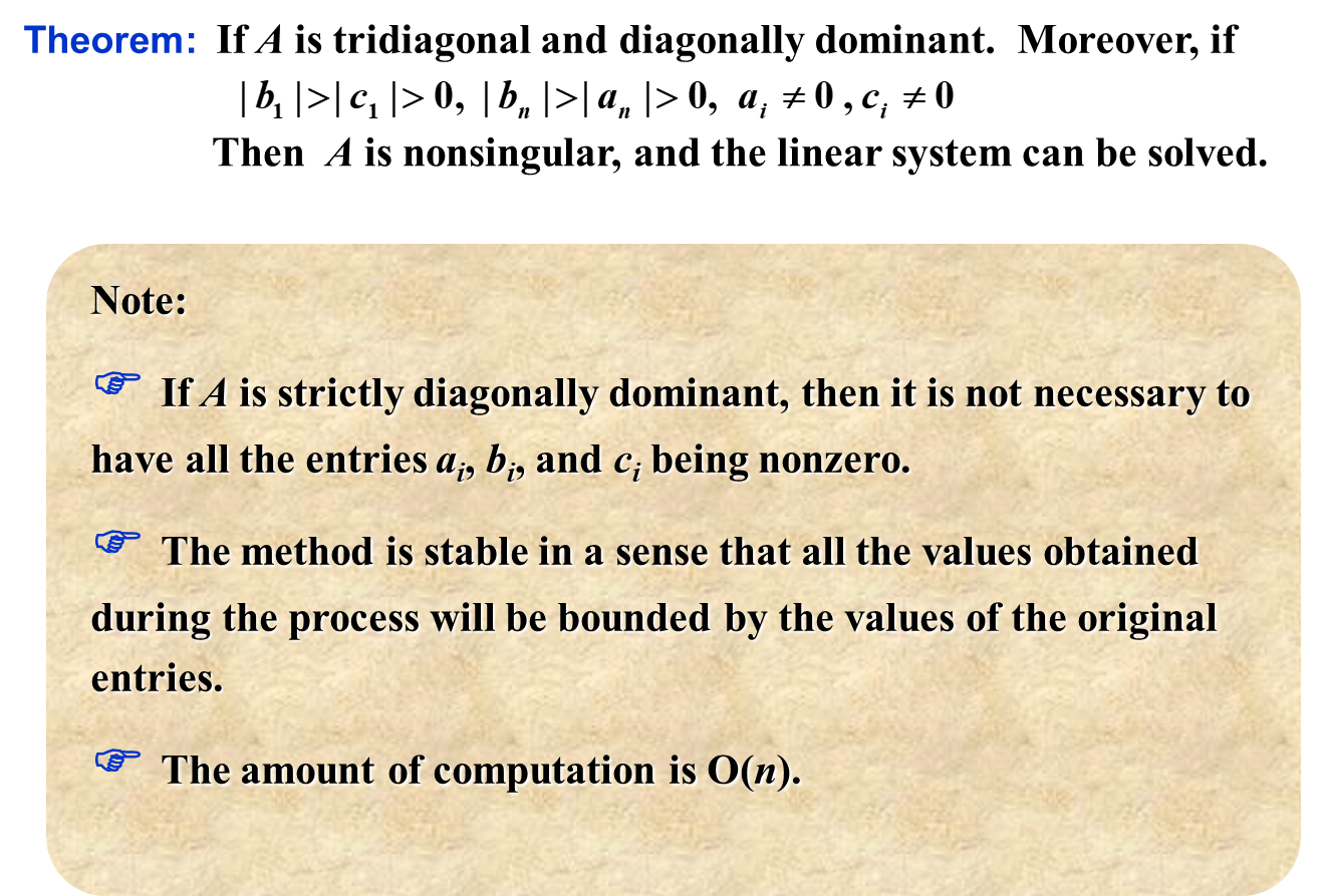
但是，前提是 \(\forall i: \alpha_i \neq 0\)。

\(\exists i: \alpha_i = 0 \iff \det(A) = 0\)。因此，能用这个方法当且仅当 \(A\) 不是奇异矩阵。
Non-singular 的充分条件：如果 A 满足上面 theorem 里面的条件，那么 \(A\) 就不是奇异矩阵，就可以这样算。

Selected Problem

使用 four digit rounding arithmetics 来求 \(\widehat H = (H^{-1})^{-1}\)，然后求 \(\|\widehat H - H \|_\infty\)

import numpy as np
from scipy.linalg import hilbert
from decimal import Decimal, getcontext

getcontext().prec = 4 # Set digit

def inv3(m4):
    iden = np.vectorize(Decimal)(np.eye(3))
    m = np.concatenate((m4.copy(), iden), axis=1)
    m[1] -= m[0] * m[1][0] / m[0][0]
    m[2] -= m[0] * m[2][0] / m[0][0]
    m[1][0] *= 0
    m[2][0] *= 0
    m[2] -= m[1] * m[2][1] / m[1][1]
    m[2][1] *= 0
    m[1] -= m[2] * m[1][2] / m[2][2]
    m[0] -= m[2] * m[0][2] / m[2][2]
    m[1][2] *= 0
    m[0][2] *= 0
    m[0] -= m[1] * m[0][1] / m[1][1]
    m[0][1] *= 0
    m[0] /= m[0][0]
    m[1] /= m[1][1]
    m[2] /= m[2][2]
    return m[:,3:6]

def hat3_cnt(m4, n):
    ret = m4.copy()
    for i in range(n):
        ret = inv3(inv3(ret))
    return ret

m4 = np.vectorize(Decimal)(hilbert(3))
m4_hat = hat3_cnt(m4, 1)

def inf_norm(x):
    x = np.vectorize(np.float32)(x)
    x_sum = np.sum(np.abs(x), axis=1)
    return np.max(x_sum)

# print(inf_norm(hat3_cnt(m4, 1) - m4))
print(inf_norm(m4_hat - m4))