Lec 4: Optimization
Note: 下面的不同 formulae 之间,加减号、常数可能会不太一样。在实际中,不同人写的书、代码里面,也不尽相同。不过这些都无关紧要。
Stochastic Gradient Descent
Normal Gradient Descent: $$ w_{t+1} = w_{t} - \alpha \nabla F(w_t) $$ where \(F(w) := \frac 1 N \sum_{i=1}^N L(x_i; y_i; w)\) is a multivariable function that take account for the whole dataset.
But actually, you can use a random minibatch of the whole set.
So, instead of \(F\), you can just use \(f\) here, where \(f := \frac 1 n \sum_{x \text{ from a random subset of size }n} L(x; y; w)\), and \(n \ll N\) or even \(n = 1\)
Problems
If the noise is big, the gradient might be really unstable, and make the descending route shape like this:
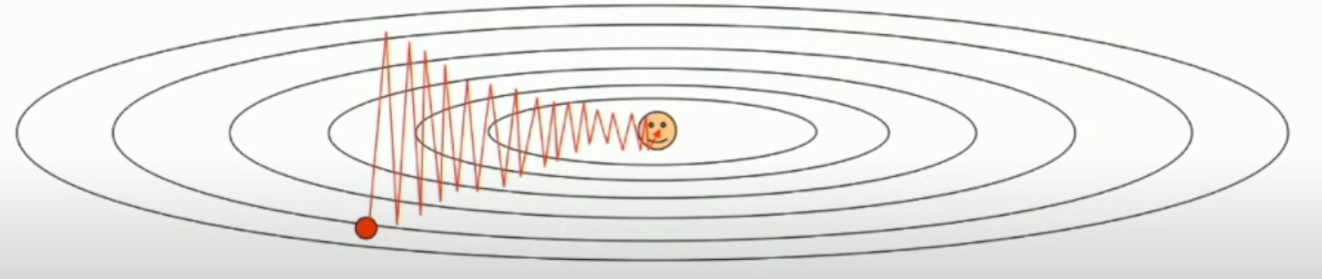
That's partly because the loss function has a high condition number.
Momentum
In the formula above, \(\rho\) is like the friction parameter (and the quicker, the more friction, the less \(\rho\)), and \(\nabla f(w_t)\) is like the force.
If you set \(\rho\) to zero, the formula degenerates to normal gradient descent.
Nesterov Momentum
We can simplify it by a change of variable \(\widetilde x_{t} := x_t + \rho v_t\), then: $$ v_{t+1} = \rho v_{t} - \alpha \nabla f(\widetilde x_t) \newline \widetilde x_{t+1} = \widetilde x_t + \alpha v_{t+1} + \rho(v_{t+1} - v_{t}) $$ You can see the difference is that Nesterov momentum has \(v_{t+1} - v_t\).
AdaGrad & RMSDrop
但是,这样的话,\(s_t\) 只增不减,因此我们需要 decay rate \(\rho\)。这就是新方法 RMSDrop: $$ s_{t+1} := \rho s_{t} + (1-\rho)\nabla f^2(w_t) \newline x_{t+1} := x_t - \frac {\alpha\nabla f(w_t)} {\sqrt{s_{t+1}} + 10^{-7}} $$ 这样,\(s_t\) 就可以自适应地增减。
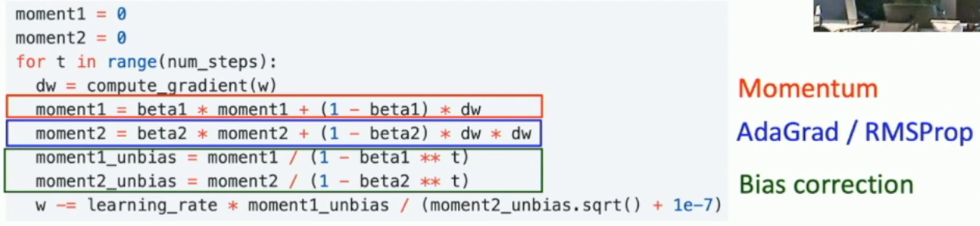
Adam
我们可以融合
- 动量
- 自适应学习率
从而得到 Adam 最优化方法(\(\sone\) 就是动量,\(\stwo\) 就是自适应变量): $$ \begin{aligned} \sone_{t+1} &:= \rone \sone_{t} + (1-\rone) \nabla f(\sone_t) \newline \stwo_{t+1} &:= \rtwo \stwo_{t} + (1-\rtwo) \nabla f^2(\stwo_t) \newline x_{t+1} &:= x_t - \frac {\alpha \sone_{t+1}}{\sqrt{\stwo_{t+1}} + 10^{-7}} \end{aligned} $$ 不过,这样还不够。因为初始的时候,如果 \(\rtwo\) 太小,那么 \(\sqrt{\stwo_{t+1}}\) 就可能会比 \(\sone_{t+1}\) 小得多。因此实际算法中,还会有一个 bias correction。
Adam in Action
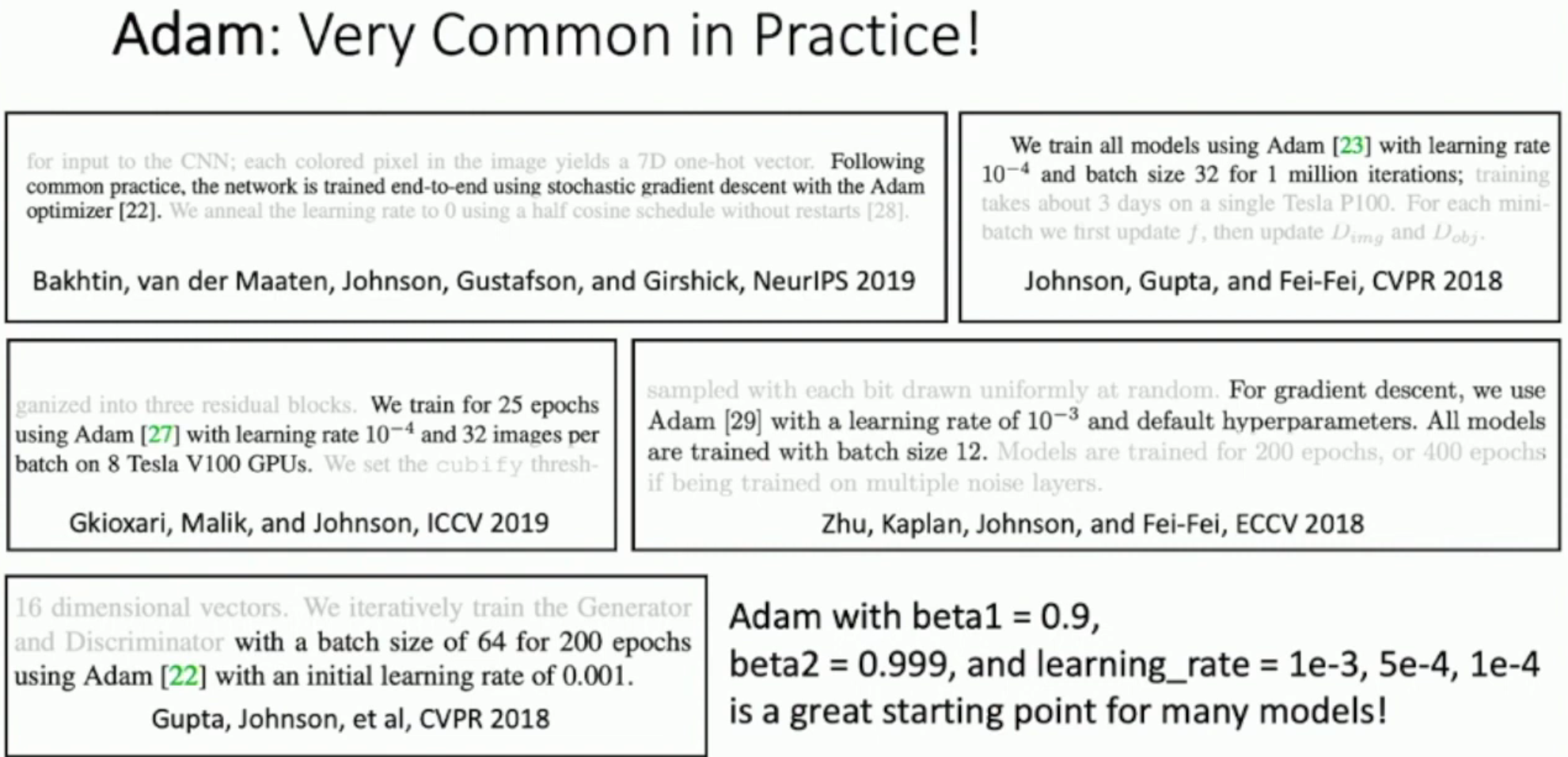
因此,Adam 优化方法,直到现在,也没有过时。
Comparison Between These Optimizers
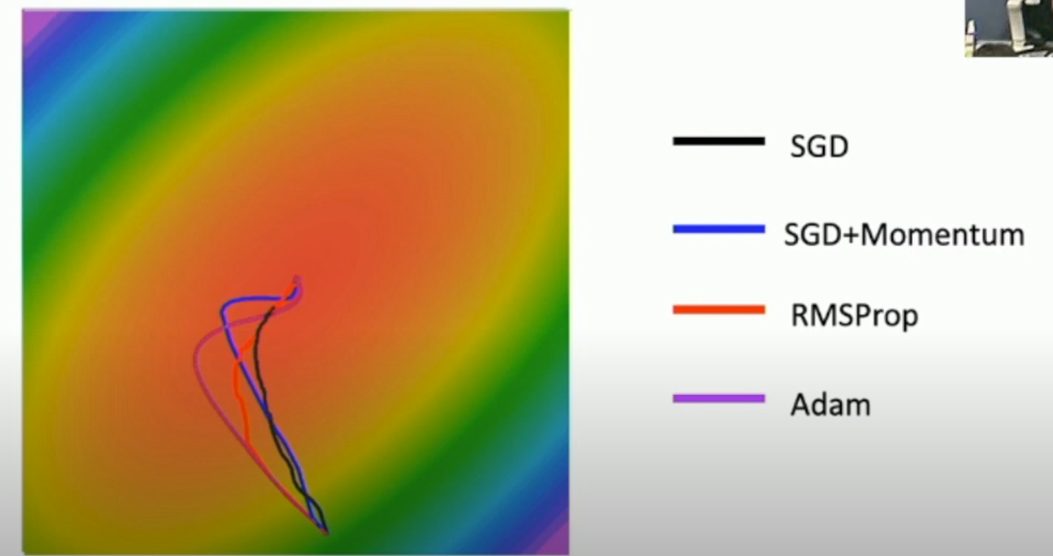
一阶优化和二阶优化
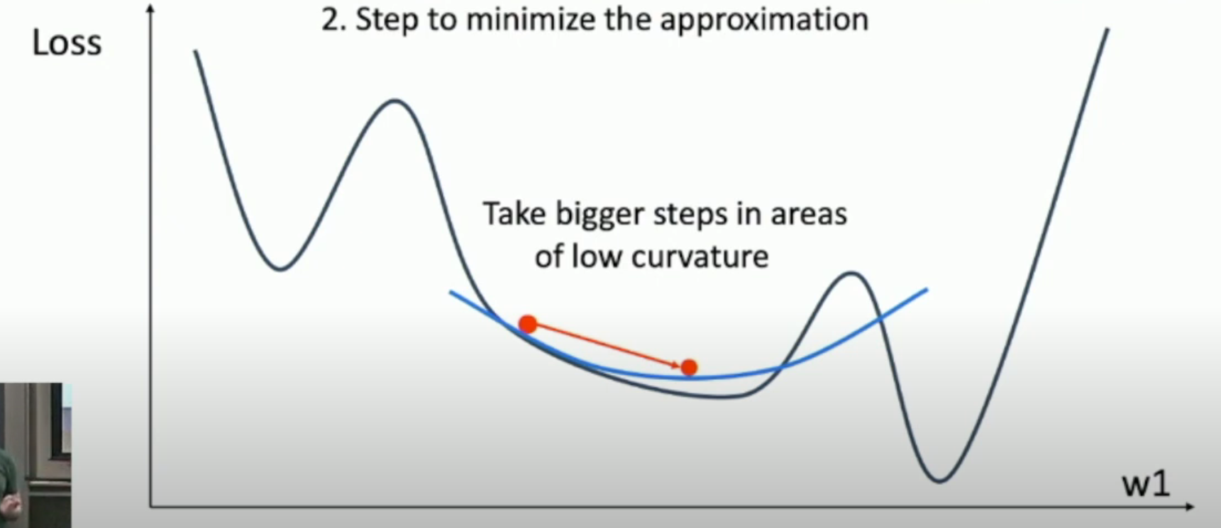
二阶优化的 robustness 往往强于一阶优化(如下图,我们如果知道了 Hessian matrix,就可以根据其得到曲率,从而适当加大 step)。
- 不过,由于 SGD+Momentum 和 AdaGrad 对过往的梯度进行了累加,从而得到了和 Hessian matrix 类似的信息。
当然,由于二阶优化涉及到了矩阵(而且还要通过矩阵的逆来求出二次曲面的极小值点,如下式),我们一般对于高维数据,不会使用二阶优化的方法。
从而,该二次曲面的最小值点就在: $$ \nabla_w L(w_0) + (w - w_0)^T \mathrm{H}_wL(w_0)= w_0 - (L(w_0)\mathrm{H}_w)^{-1}\nabla_wL(w_0) $$
- 注意算式中要对 Hessian 阵取逆。由于 Hessian 矩阵是稠密矩阵,因此没什么好方法,一般而言,复杂度就是在 \(\mathcal O(n^3)\) 这个量级的。
In Practice
- Adam is a good default choice in many cases. SGD+Momentum can outperform Adam but may require more tuning
- If you can afford to do full batch updates and the dimension is low, then try out L-BFGS (and don't forget to disable all sources of noise)