Lec 21-22: Animation
弹簧-质点系统(Mass Spring System)
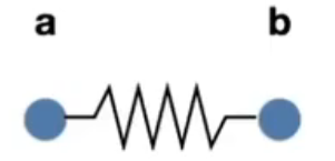
对于如上的弹簧,我们考虑二阶力(弹簧势能)和一阶力(摩擦力):
-
二阶力 $$ \begin{aligned} \boldsymbol f_{a \to b} &= k_s \frac{\boldsymbol {b-a}}{\lVert\boldsymbol{b-a}\rVert}(\lVert\boldsymbol{b-a}\rVert - l) =k_s \widehat{\boldsymbol {b-a}}(\lVert\boldsymbol{b-a}\rVert - l) \newline \boldsymbol f_{b \to a} &= -\boldsymbol f_{a \to b} \end{aligned} $$
-
其中,\(l\) 是 rest length
-
一阶力 $$ \begin{aligned} \boldsymbol f_{b} = -k_d (\widehat{\boldsymbol {b-a}} \cdot (\boldsymbol{\dot b - \dot a}) )\widehat{\boldsymbol {b-a}} \newline \boldsymbol f_{a} = -\boldsymbol f_{b}
\end{aligned} $$ -
括号里就是 a, b 相对速度在弹簧方向上的大小。
例子:布料
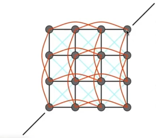
如图,布料具有
- (各向同性)抗剪切
- 抗弯折
- ……
的特性。因此,横平竖直的弹簧系统肯定是不行的。
为了抗剪切,我们加入了对角线的弹簧;为了抗弯折,我们加入了 skip connection(也就是如图长度为 2 的长弹簧)。
从而,我们得到了可以近似模拟布料的 mass spring system。
粒子系统
我们可以将一个系统近似为粒子之间的相互作用。
每个粒子的运动都由一系列物理/非物理的力所决定。
It's a popular technique in graphics and games, in the sense that it's
- Easy to understand, implement
- Scalable: fewer particles for speed, more for higher complexity
but it does have challenges
- May need many particles (e.g. fluids)
- May need acceleration structures (e.g. to find nearest particles for interactions)
Particle System Animations
For each frame in animation - [If needed] Create new particles - Calculate forces on each particle - Update each particle’s position and velocity - [If needed] Remove dead particles - Render particle
Particle System Forces
Attraction and repulsion forces - Gravity, electromagnetism, … - Springs, propulsion, … Damping forces - Friction, air drag, viscosity, … Collisions - Walls, containers, fixed objects, … - Dynamic objects, character body parts, …
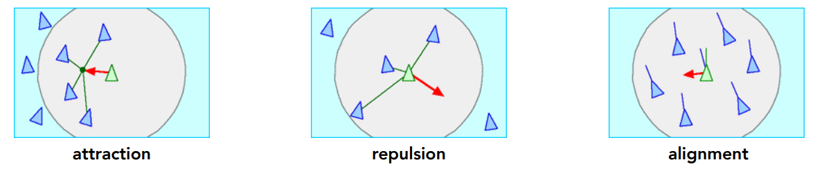
例子:bird flock simulation (as ODE)
Model each bird as a particle Subject to very simple forces:
- attraction to center of neighbors
- repulsion from individual neighbors
- alignment toward average trajectory of neighbors
数值模拟——欧拉方法
欧拉方法很广,可以分为
-
直接欧拉法(i.e. naive Euler method),\(\bxtt = \bxt + \bv(\bxt) \Dt\)
-
中点法 $$ \begin{aligned} \newcommand{\bxmid}{\bxt + \bv(\bxt)\Dt / 2} \bx_{mid} &= \bxmid \newline \bxtt &= \bxt + \bv(\bx_{mid}) \Dt = \bxt + \bv(\bxmid) \Dt \end{aligned} $$
-
中点法很多情况下等价于一个抛物线
-
隐式欧拉法
通过求解方程(\(\bxtt\) 是未知数) $$ \begin{aligned} \bxtt = \bxt + \Dt ~\dbxtt = \bxt + \Dt ~\bv(\bxtt) \end{aligned} $$ 我们可以通过牛顿迭代法等方法求出 \(\bxtt\) 的值
-
通常,隐式欧拉法比直接(显式)欧拉法更加稳定
-
Runge-Kutta Families
这是一系列高阶优化方法的集合,很适合用作非线性的情况。