Lec 14: Ray Tracing 2
加速结构
上一节课,我们使用了 Bounding Volume 减小了检测光线与物体碰撞的计算量。本节课,我们进一步优化。
Build Acceleration Grid
将 Bounding Volume 划分成一定数量的格子。每个格子或者与 Bounding Volume 内某物体相交,或者不相交。我们计算出光线碰到的格子,如果格子存在某物体,那么就进一步求交,否则就还是没碰到。
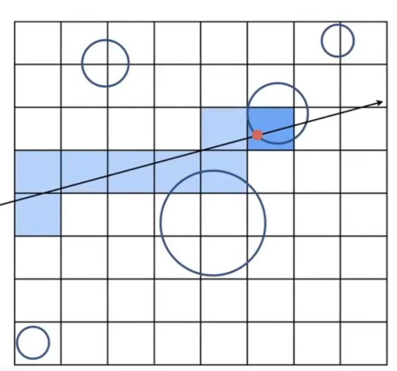
- 如上图所示,光线在深蓝色格子处,碰到了圆形物体,从而只用与该圆形物体求交。
网格分辨率
格子太稀疏,固然判断不好;太密集,计算量也会较大。一个好用的 heuristic 是:
- \(\#cells = C * \#objs\)
- $C \approx 27 $ in 3D
网格适用范围
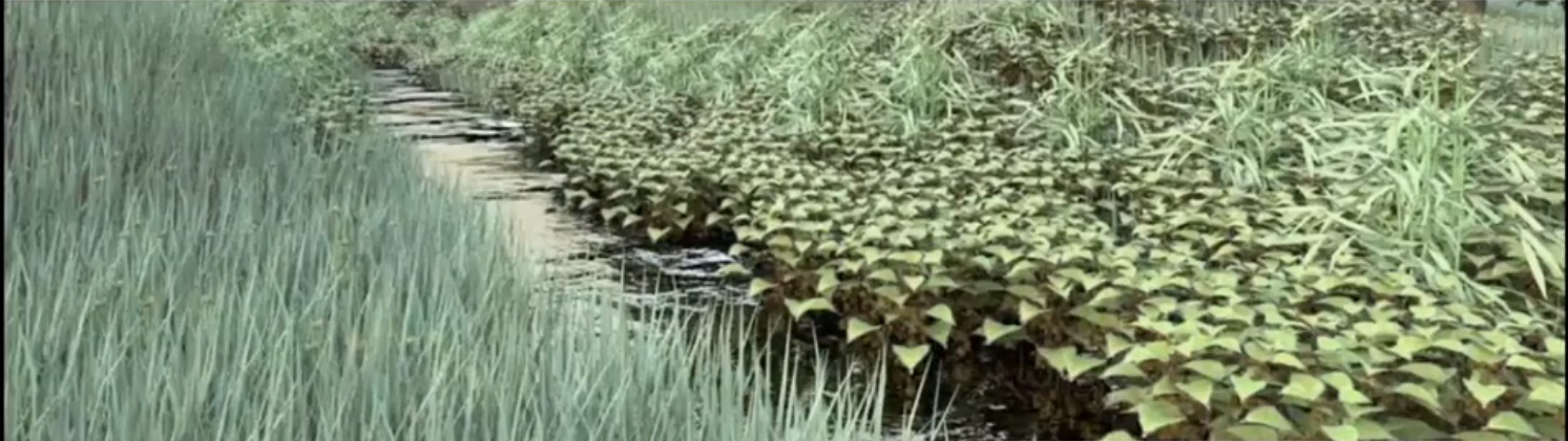
Grids work well on large collections of objects that are distributed evenly in size and space
But work badly on those distributed unevenly in size and space
- "teapot in a stadium" problem
Spatial Partitions
为了改进网格的分割,我们使用 spatial partitions 的方式,也就是采用不均匀划分的方式,。
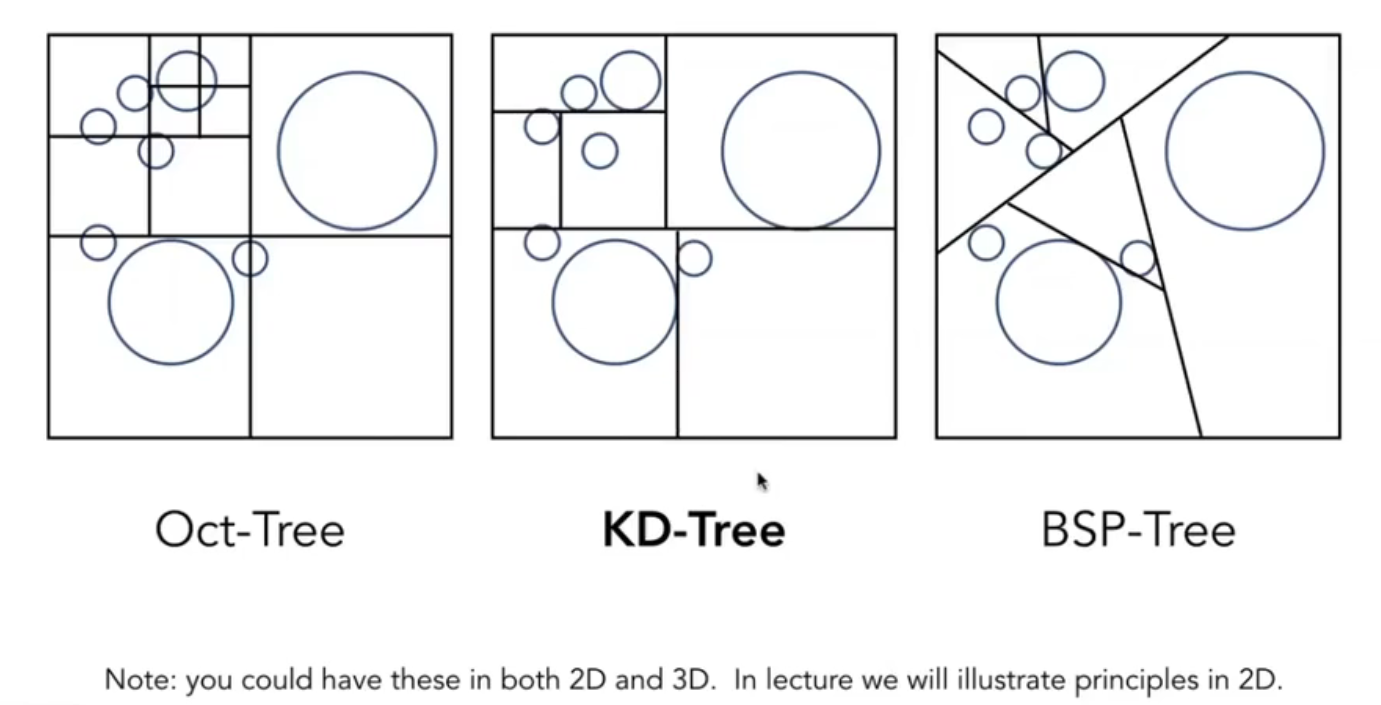
由于 Oct-Tree (or Quad-Tree in 2D plane) 每一次划分都必须有 8 叉,复杂度太高,我们并不愿意使用。
由于 BSP-Tree 每一次划分都是超平面,在维度较高时,超平面判交计算起来困难,因此我们在这里也不介绍。
我们在这里介绍 KD-Tree。
KD-Tree: Introduction
KD-Tree 在 2D 上交替地沿着 x-axis 和 y-axis 进行划分,在 3D 上交替地以 x-, y-, z-axis 作为法线进行划分。
图例:
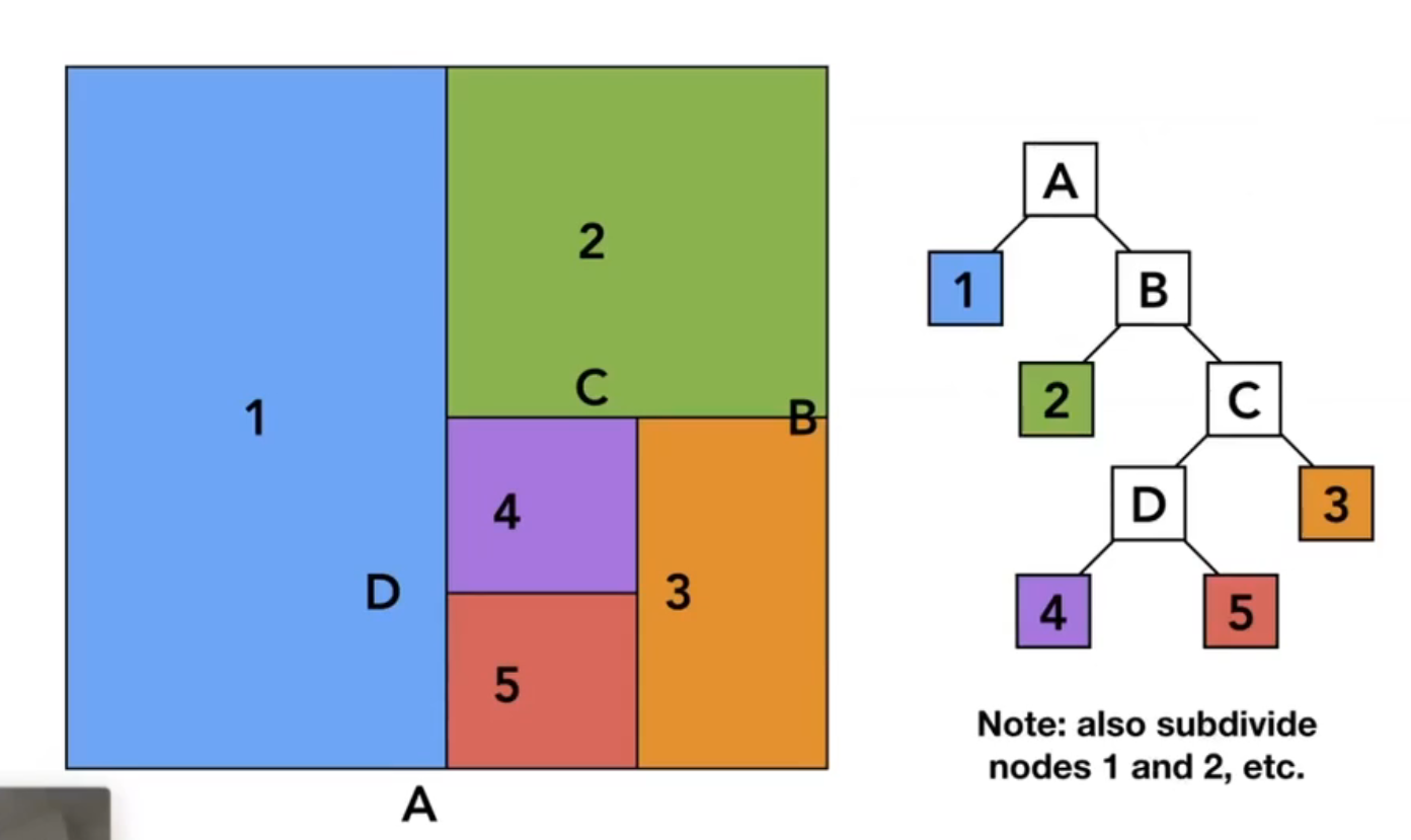
KD-Tree: Data Structure
在 KD-Tree 中,中间的节点储存:
- split axis: x-, y-, or z-axis (in 3D)
- split position: coordinate of split plane along axis
- children
叶子节点储存:
- list of objects (that intersect with the leaf)
KD-Tree: Compute The Intersections
我们递归地进行求交测试。
如果光线与某个
-
任意节点无交点,则直接返回,不用理会这个节点的潜在的子节点或 list of objects 了
-
非叶子节点有交点,则继续递归计算是否与其两个子节点有交点
- 叶子节点有交点,则对 list of objects 逐一进行求交
最后找到 \(t\) 最小的交点以及对应物体,即为所求。
KD-Tree: Problems
有两个问题:
- 判断三角形是否与立方体相交,算法上繁琐
- 一个物体可能出现在多个叶子节点里,性质不好
所以,目前用来得越来越少。
Object Partition
换一种思路:与其把空间分成两份,然后再分别求两个空间里的物体;不如把物体分成两份,然后再分别求两份物体的 bounding volume,如图:
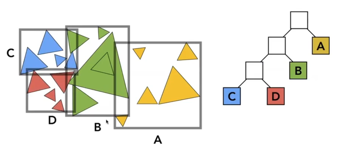
从而:
- 通过三角形反求 bounding volume,简单直观
- i.e. 求最大值即可
- 一个物体只可能出现在一组中,性质好
解决了上述问题。
这个方法被称为 Bounding Volume Hierarchy。
BVH: Algorithm
算法思想很简单:
- 将一组物体分为两部分
- 将这两部分重新求 bounding volume
- 如此递归下去,直至每组物体的物体个数少于临界值
其中,实现起来最难的部分,就是如何划分
BVH: How To Partition?
- Heuristic #1: Always choose the longest axis in node
- 沿着最长轴进行划分,从而使得 bounding volume 比较均匀
- Heuristic #2: Split the node at the median object
- 找中点(使用三路快排)
- Heuristic #3: Stop when the node contains few elements
Basic Radiometry
Terms
Radiant Energy and Flux
Definition: Radiant flux (power) is the energy emitted, reflected, transmitted or received, per unit time. $$ \Phi \equiv \frac{\mathrm dQ}{\mathrm dt} [\text{W = Watt}] [\text{lm = lumen}]^ * $$
- 实际上,watt 并不是 lumen。在 old days,100 watt 的白炽灯可以发出 400 * 3.14 lumen 的光线,对应的光强就是 100 cd。现在的灯的效率更高了,所以 1 watt 可以发出更多的光。
Radiant Intensity
Definition: The radiant (luminous) intensity is the power per unit solid angle emitted by a point light source. $$ I(\omega) = \frac {\mathrm d \Phi} {\mathrm d\omega} $$
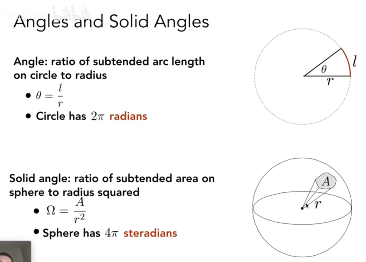
Angles and Solid Angles
Intensity of Uniformly Radiating Point Light Source
假如一个点光源均匀发光,那么: $$ I = \frac{\phi}{4\pi} $$ 因为球面的立体角为 \(4\pi\)。
Differential Solid Angles
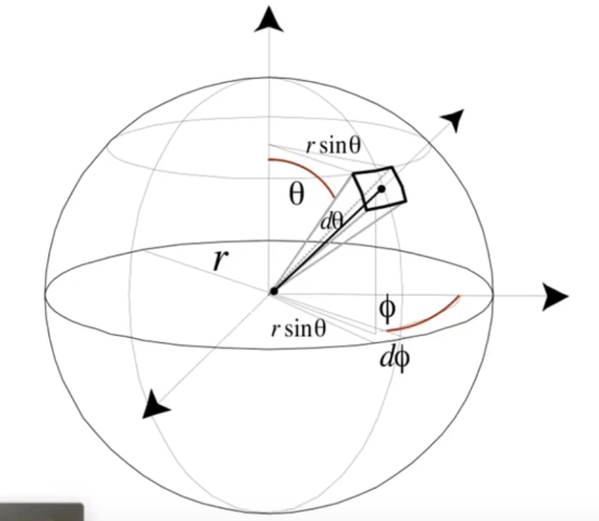
因此,有
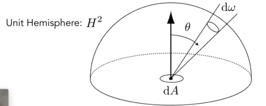
Irradiance
Definition: The irradiance is the power per (perpendicular/projected) unit area incident on a surface point.
区分:
- irradiance 是 power per unit area
- intensity 是 power per solid angles
- 前者会随着 \(r\) 的增大而减小,后者在光照均匀的前提下,是与 \(r\) 无关的。
- 前者是被照物体的属性,后者是光源的内禀属性。
Radiance
Definition: The radiance (luminance) is the power emitted, reflected, transmitted or received by a surface, per unit solid angle, per projected unit area. - 其实,radiance 还有另一层意义:人眼对发光体或被照射物体表面的发光或反射光强度实际感受的物理量
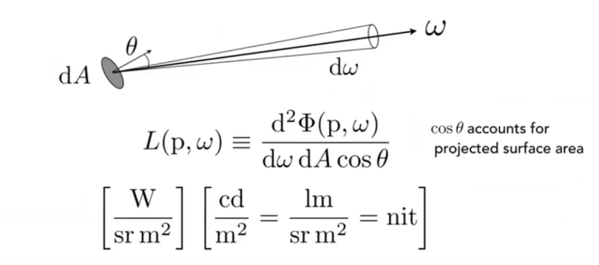
根据单位制,我们可以考虑 radiance 为
- Intensity per unit area
- Irradiance per solid angle
对于 irradiance per solid angle,其物理意义是:接受光照的物体,单位面积上,会接受一定的 radiant flux,也就是 irradiance。而这 irradiance,是来自四面八方的积分,对于某个立体角的方向,其贡献就是 radiance。
对于 Intensity per unit area,其物理意义是:发出光照的物体,往某个确定的定向立体角 \(\mathrm d \vec \omega\) 发射的光照一共是一定的 intensity。而这 intensity,是各个面积微元的积分,对于某个面积微元而言,其贡献就是 radiance。
简单来说:irradiance 和 radiance,差的就是方向性。
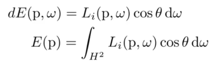
Relations Between Irradiance and Radiance
Irradiance: total power received by area \(\mathrm d A\) Radiance: power received by area \(\mathrm dA\) from "direction" \(\mathrm d\omega\)
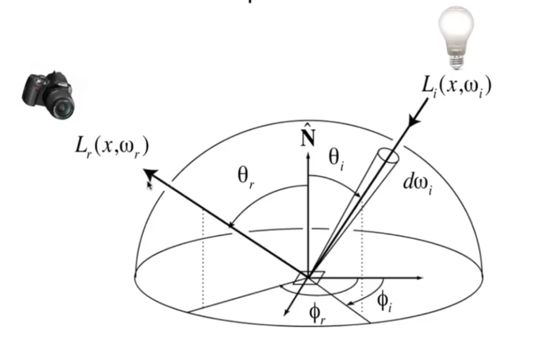
Reflection at a Point
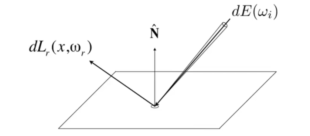
如图,从一个定向立体角入射的 radiance,会依照某种函数分配到其它各个立体角。
Differential irradiance incoming: \(\mathrm dE(\omega_i) = L(\omega_i) \cos\theta_i \mathrm d\omega_i\)
BRDF
The Bidirectional Reflectance Distribution Function (BRDF) represents how much light is reflected into each outgoing direction \(\omega_r\) from each incoming direction
$$
f_r(\omega_i \to \omega_r) = \frac{\mathrm dL_r(\omega_r)}{\mathrm dE_i(\omega_i)} = \frac{\mathrm dL_r(\omega_r)}{L_i(\omega_i)\cos\theta_i\mathrm d\omega_i} \left[\frac 1 {\operatorname{sr}}\right]
$$
为了计算一个方向上的 \(L_r\): $$ L_r(\mathbf p, \omega_r) = \int_{H^2} f_r(\mathbf p, \omega_i \to \omega_r) L_i(\mathbf p, \omega_i) \cos\theta_i \mathrm d\omega_i $$ 我们将所有入射方向到这个出射方向的 \(f_r\) 积分起来。
渲染方程
对于自身会发光的物体,还要加上自身的 radiance。从而,最终的方程为: $$ L_r(\mathbf p, \omega_o) = L_e(\mathbf p, \omega_o) + \int_{\Omega^+} L_i(\mathbf p, \omega_i) f_r(\mathbf p, \omega_i, \omega_o) (\mathbf n \cdot \omega_i) \mathrm d\omega_i $$ 其中,\(\Omega^+\) 指的是上半球。
线性算子方程
渲染方程可以进一步简化: $$ \begin{aligned} l(u) &= e(u) + \int_{\Omega^+} l(v) K(u,v) \mathrm dv \ &\text{where } K(u,v) = (\mathbf n \cdot u) f_r(\mathrm p, v, u) \end{aligned} $$ 对于某一点 \(\mathbf p\) 而言,可以把原方程转换成 Fredholm integral equation。
从而,可以进一步转换成: $$ L = E + KL $$ 其中,\(K\) 就是函数空间上的一个线性算子(因为 \(\int_{\Omega^+} l(v) K(u,v) \mathrm dv\) 也是关于 \(u\) 的一个函数,再加上积分的双线性性,因此可以这样说)。
从而: $$ \begin{aligned} (I-K) L &= E \ L &= (I - K)^{-1} E \ &= (I + K + K^2 + K^3 + \cdots) E \ &= (\sum_{i=0}^\infty K^i) E \end{aligned} $$ 也就是说: $$ l(u) = e(u) + \int_{\Omega^+} e(v) K(u,v) \mathrm dv $$ 直观意义上,就是将无限多次的折射相加,从而得到真实的光照。
实际上,我们无法做到无限多次,只能做到有限多次,从而只能进行固定次数的迭代。
- 当然,还是比 rasterization 更好。毕竟 rasterization 一般只能做到 \(L = E + KE\)。
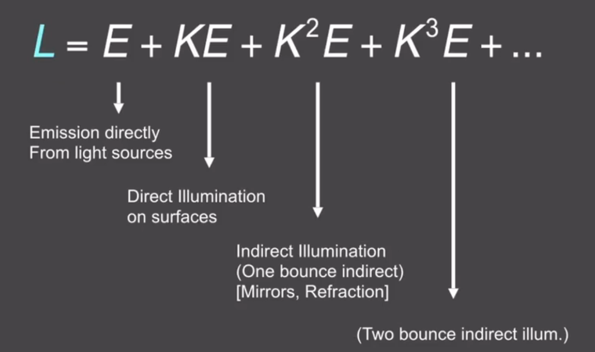
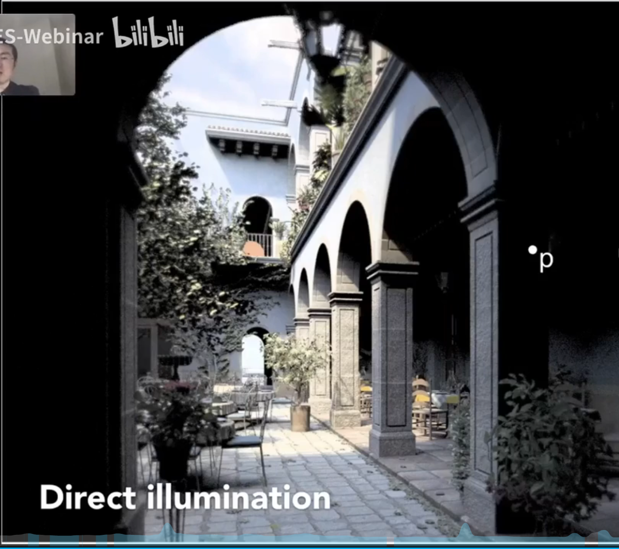
渲染效果
直接光照,\(L = E + KE\)
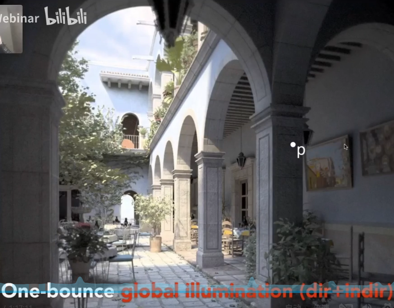
一次间接光照:\(L = E + KE + K^2 E\)
两次间接光照(i.e. 最多弹射三次):\(L = E + KE + K^2E + K^3E\)
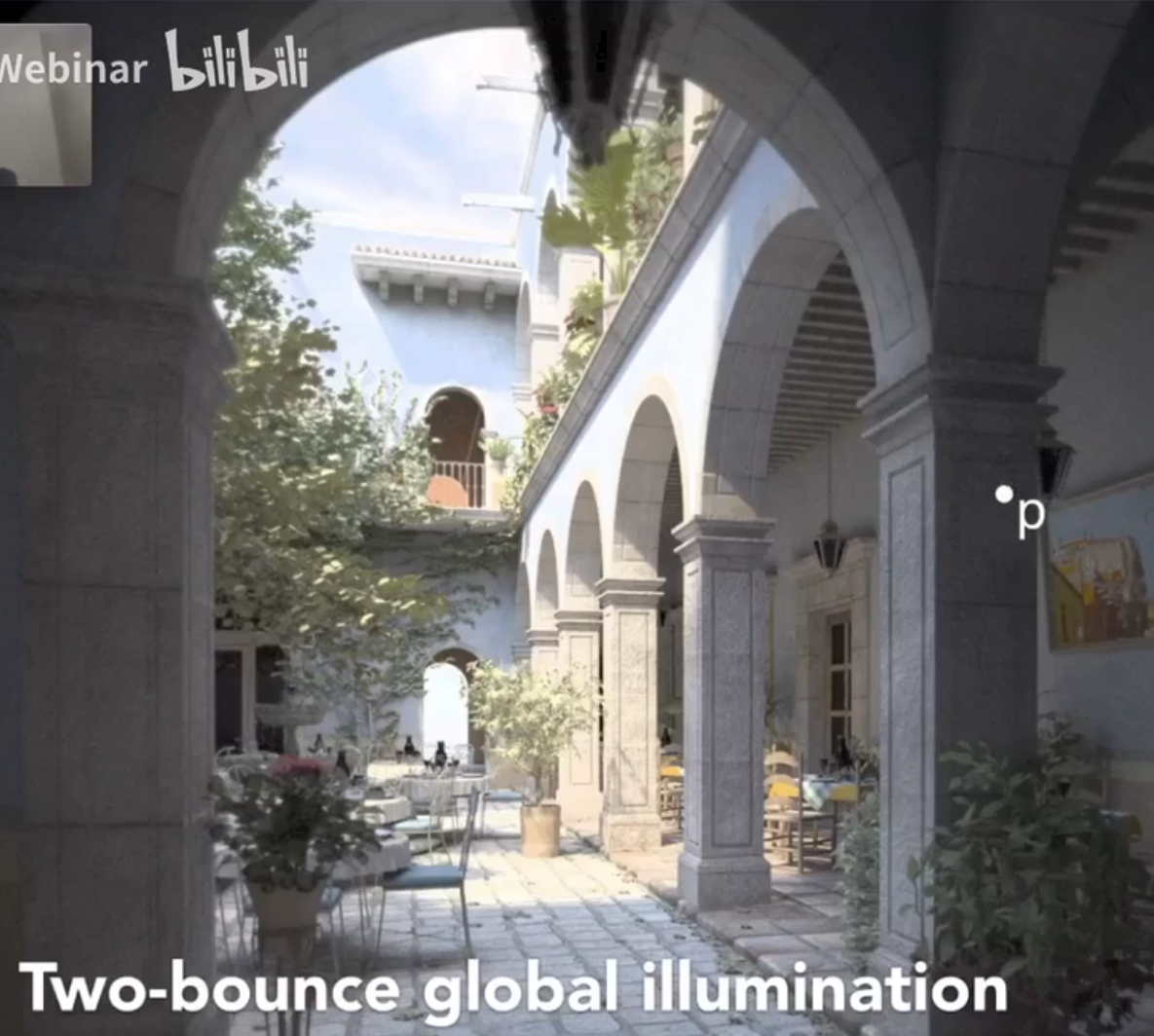
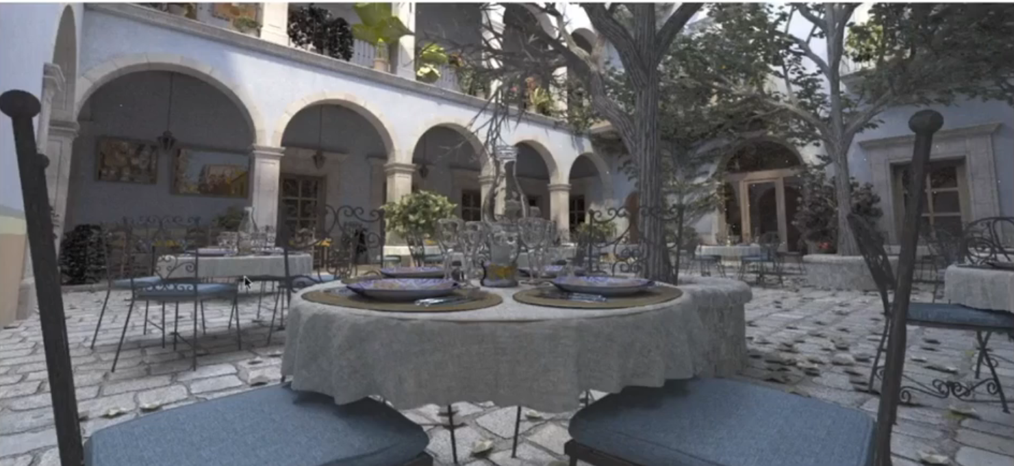
四次(i.e. 最多弹射五次):\(L = E + KE + K^2E + K^3E + K^4E + K^5E\)
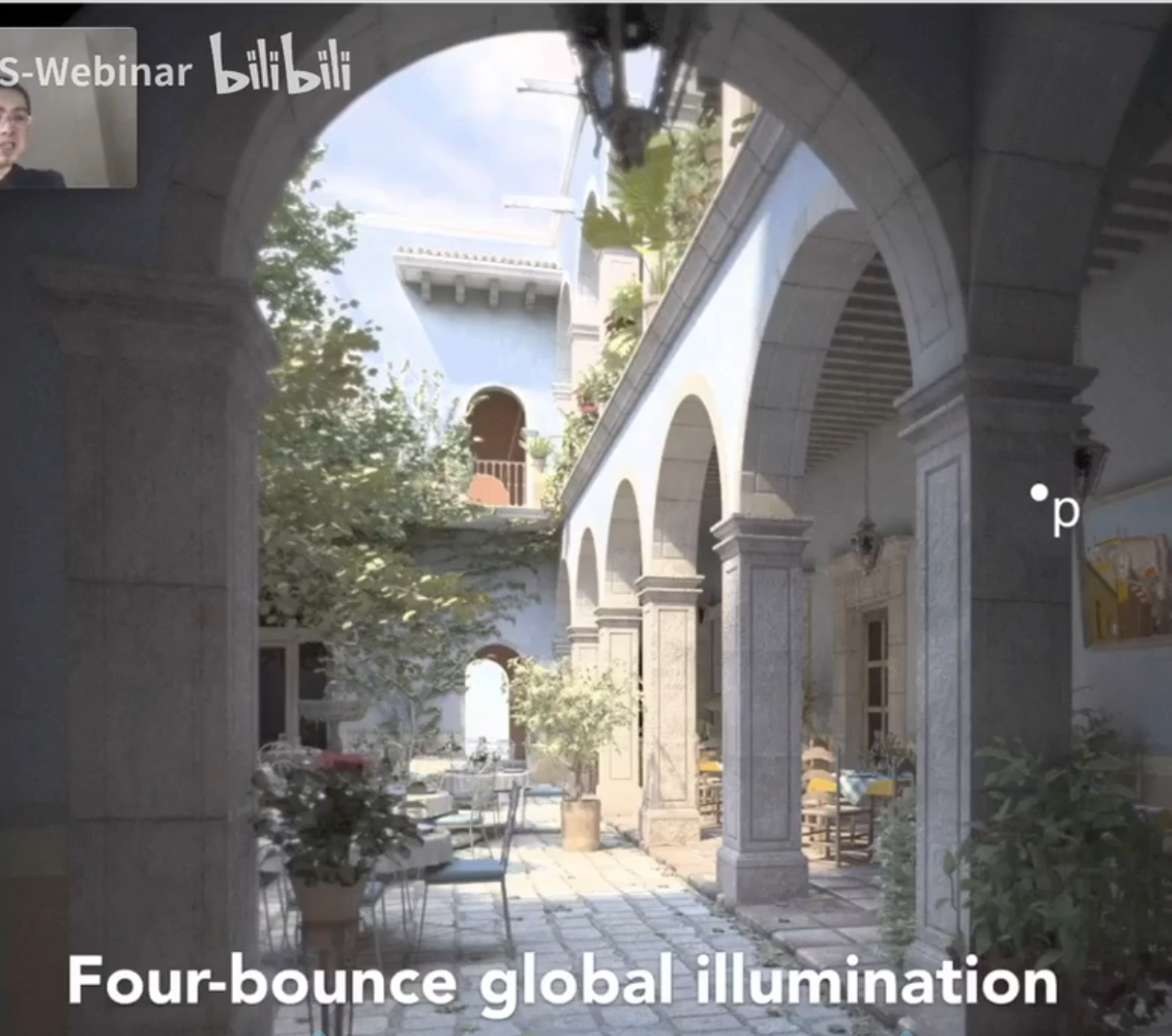
- 注意,弹射五次后,吊灯的玻璃亮了。这是因为一个玻璃需要两次弹射,因此,两层玻璃需要四次弹射。所以,两次间接光照只有三次弹射,还差一次,所以玻璃是暗的。
Monte Carlo Sampling
\(L_r(\mathbf p, \omega_o) = L_e(\mathbf p, \omega_o) + \int_{\Omega^+} L_i(\mathbf p, \omega_i) f_r(\mathbf p, \omega_i, \omega_o) (\mathbf n \cdot \omega_i) \mathrm d\omega_i\)
对于这个方程,我们希望求出的就是 \(L_r(\mathbf p, \omega_o)\),未知量是 \(L_i(\mathbf p, \omega_i)\)。
如果我们有一个随机向量 \(\mathbf \xi \in \Omega^+\),那么: $$ \mathbb E \left[\frac{f(\mathbf\xi)}{p_\mathbf\xi(\mathbf\xi)}\right] = \int_{\Omega^+} p_\mathbf\xi(\mathbf x) \frac{f(\mathbf x)}{p_\mathbf\xi(\mathbf x)} \mathrm d\mathbf x = \int_{\Omega^+} f(\mathbf x) \mathrm d\mathbf x $$ 从而,我们可以通过多次采样的方式,来近似 RHS。
在这里,我们不妨直接让 \(\mathbf \xi\) 在 \(\Omega^+\) 上均匀采样。
从而: $$ \int_{\Omega^+} L_i(\mathbf p, \omega_i) f_r(\mathbf p, \omega_i, \omega_o) (\mathbf n \cdot \omega_i) \mathrm d\omega_i \approx \frac 1 N \sum_{i = 1}^N L_i(\mathbf p, \xi_i) f_r(\mathbf p, \xi_i, \omega_o) (\mathbf n \cdot \xi_i) $$
我们使用递归的方法来不断求出各个物体 \(L_i\)(因此不考虑实际限制的话,深度可以无限大)。伪代码如下:
shade(p, wo):
    Randomly choose N directions wi~dist
    Lo = 0.0
    for each wi:
        Trace a ray r(p, wi)
        If ray r hit the light x
            Lo += (1 / N) * L_i(x, -wi) * f_r * cosine / pdf(wi) // if dist=Uniform(Omega), pdf = 1 / (2*pi)
        Else If ray r hit an object at q
            Lo += (1 / N) * shade(q, -wi) * f_r * cosine / pdf(wi)
    Return Lo
仍然有两个问题:
- \(N>2\) 的时候,如果深度过于大,很容易造成指数爆炸。
- 深度本身没有限制,在一些特殊情况下可能会造成死循环
解决方法:
- 令 \(N=1\)(我们采用的方法)
- 采用 \(\epsilon\)-stop 的方式(或称 Russian Roulette)。也就是:\(\mathbb E \left[\frac{f(\mathbf\xi)}{p_\mathbf\xi(\mathbf\xi)}\right] = \mathbb E \left[X_{1-\epsilon}\frac{f(\mathbf\xi)}{p_\mathbf\xi(\mathbf\xi)(1-\epsilon)}\right]\) 其中,\(X_{1-\epsilon}\) 就是有 \(\epsilon\) 的概率等于 0 的、独立的零一随机变量
经过两次修改,代码如下:
shade(p, wo):
    Randomly choose ksi~Uniform(0,1)
    if (ksi < epsilon) return 0.0.

    Randomly choose ONE direction wi~dist
    Lo = 0.0
    Trace a ray r(p, wi)
    If ray r hit the light x
        Return L_i(x, -wi) * f_r * cosine / pdf(wi) / (1 - epsilon) // if dist=Uniform(Omega), pdf = 1 / (2*pi)
    Else If ray r hit an object at q
        Return shade(q, -wi) * f_r * cosine / pdf(wi) / (1 - epsilon)
仍然有一个问题:如何控制采样方差?
一个好的 \(p_\xi\),应该和 \(f\) 的形状相似。也就是说,我们应该尽量在有光的方向进行采样。
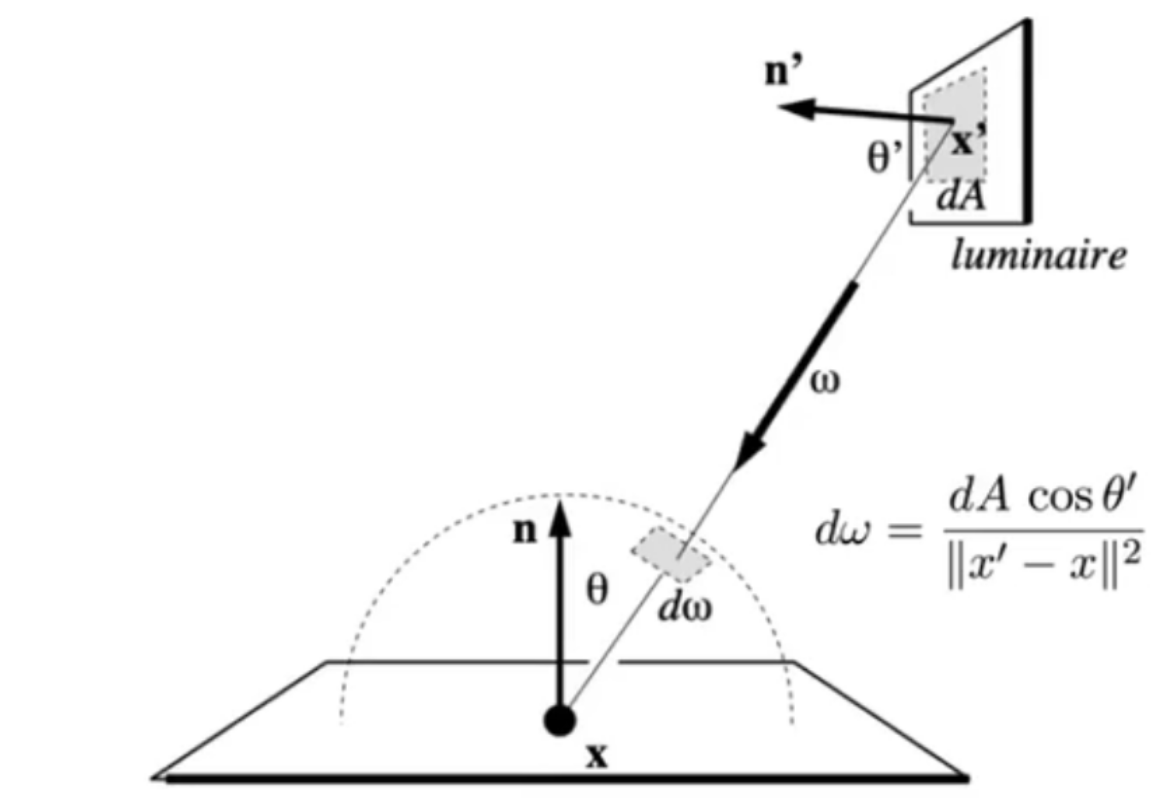
对于 ray r hit the light x 的情况,其实我们不如直接在光源上进行均匀采样,然后再把这个随机变量的 pdf 转换成立体角的 pdf。
假设只有一个光源,且没有其它反光物体。令 \(\xi' \sim \operatorname{Uniform}(A)\),从而: $$ \begin{aligned} \lVert x'-x\rVert^2 \mathrm d\omega &= \cos \theta' \mathrm d A \ \frac{\mathrm d A}{\mathrm d\omega} &= \frac{\lVert x'-x\rVert^2}{\cos \theta'} \end{aligned} $$ 从而, $$ p_\xi(\mathbf x) = p_{\xi'}(\mathbf y) \frac{\lVert x'-x\rVert^2}{\cos \theta'} $$ 其中,\(\mathbf y\) 就是与立体角坐标 \(\mathbf x\) 对应的面积坐标。
注意:
- 如果有多个光源,我们可以分别进行采样,然后累加到该点的光照 \(L_o\)。
- 对于非直接光源,我们还是采用原先的在半球上均匀随机采样的方法。
- 也就是说,我们分别讨论直接光源和反射光源,前者直接在光源(平面)上采样,后者还是在原半球进行采样
- 最后,还要判断一下视线和直接光源之间有没有遮挡物。如果有的话,就
=0.0。
代码:
shade(p, wo)
    # Contribution from the light source.
    Uniformly sample the light at x’ (pdf_light = 1 / A)
    If no blockings within the path:
        L_dir = L_i * f_r * cos θ * cos θ’ / |x’ - p|^2 / pdf_light
    Else:
        L_dir = 0.0

    # Contribution from other reflectors.
    L_indir = 0.0
    Test Russian Roulette with probability P_RR
    Uniformly sample the hemisphere toward wi (pdf_hemi = 1 / 2pi)
    Trace a ray r(p, wi)
    If ray r hit a non-emitting object at q
        L_indir = shade(q, -wi) * f_r * cos θ / pdf_hemi / P_RR

    Return L_dir + L_indir