五(下)
本文由 简悦 SimpRead 转码, 原文地址 zhuanlan.zhihu.com
代码
好了,我们在第五章上半部分基本上已经涵盖了计算持续同调的概念框架。让我们编写一些代码来计算实际数据的持续同调。我不会花太多精力解释所有的代码以及它的原理,因为我更关心实际和直观的解释,所以你可以自己写算法。我尝试添加行内的注释,这应该有帮助。也请记住,因为这一系列文章都是有科普目的的,这些算法和数据结构可能不会很有效,但会很简单。我希望可以针对一些点写一篇后续文章,演示如何高效使用这些算法和数据结构的版本。
让我们首先使用第四章中所写的代码构造一个简单的单纯复形结构。
#for example... this is with a small epsilon, to illustrate the presence of a 1-dimensional cycle
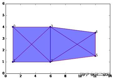
graph = SimplicialComplex.buildGraph(raw_data=data, epsilon=5.1)
ripsComplex = SimplicialComplex.rips(nodes=graph[0], edges=graph[1], k=3)
SimplicialComplex.drawComplex(origData=data, ripsComplex=ripsComplex, axes=[0,7,0,5])
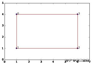
所以我们的单纯复形是一个盒子。显然它有 \(1\) 个连接分量和 \(1\) 维的环。如果你持续增大 \(\epsilon\) ,那么盒子会被 “填满”,而我们会得到一个最大单形——所有四个点相连形成一个 \(3\) 维单形(四面体)
接下来,我们将对第四章的代码做一些修改,让它能够处理滤流复形的计算过程,而不只是基本的单纯复形而已。
所以我准备撸一堆代码在下面,并直观的描述一下每个函数都在做什么的。buildGraph 函数和之前一样。但是我们也有一些新的函数:ripsFiltration,getFilterValue,compare 和 sortComplex。
ripsFiltration 函数接收从 buildGraph 输出的图对象和最大维度 k(即我们要计算的单形的维度),并返回通过过滤值储存的单纯复形对象。过滤值按照上面描述的那样定义。我们有 sortComplex 方法,它能接收复形和过滤值,返回复形的排序。
所以我们之前的单纯复形函数和 ripsFiltration 函数唯一的不同是后者还要维每个单形生成过滤值,并根据域流对单形进行全序的排序。
def euclidianDist(a,b): #this is the default metric we use but you can use whatever distance function you want
    return np.linalg.norm(a - b) #euclidian distance metric


#Build neighorbood graph
def buildGraph(raw_data, epsilon = 3.1, metric=euclidianDist): #raw_data is a numpy array
    nodes = [x for x in range(raw_data.shape[0])] #initialize node set, reference indices from original data array
    edges = [] #initialize empty edge array
    weights = [] #initialize weight array, stores the weight (which in this case is the distance) for each edge
    for i in range(raw_data.shape[0]): #iterate through each data point
        for j in range(raw_data.shape[0]-i): #inner loop to calculate pairwise point distances
            a = raw_data[i]
            b = raw_data[j+i] #each simplex is a set (no order), hence [0,1] = [1,0]; so only store one
            if (i != j+i):
                dist = metric(a,b)
                if dist <= epsilon:
                    edges.append({i,j+i}) #add edge if distance between points is < epsilon
                    weights.append(dist)
    return nodes,edges,weights

def lower_nbrs(nodeSet, edgeSet, node): #lowest neighbors based on arbitrary ordering of simplices
    return {x for x in nodeSet if {x,node} in edgeSet and node > x}

def ripsFiltration(graph, k): #k is the maximal dimension we want to compute (minimum is 1, edges)
    nodes, edges, weights = graph
    VRcomplex = [{n} for n in nodes]
    filter_values = [0 for j in VRcomplex] #vertices have filter value of 0
    for i in range(len(edges)): #add 1-simplices (edges) and associated filter values
        VRcomplex.append(edges[i])
        filter_values.append(weights[i])
    if k > 1:
        for i in range(k):
            for simplex in [x for x in VRcomplex if len(x)==i+2]: #skip 0-simplices and 1-simplices
                #for each u in simplex
                nbrs = set.intersection(*[lower_nbrs(nodes, edges, z) for z in simplex])
                for nbr in nbrs:
                    newSimplex = set.union(simplex,{nbr})
                    VRcomplex.append(newSimplex)
                    filter_values.append(getFilterValue(newSimplex, VRcomplex, filter_values))

    return sortComplex(VRcomplex, filter_values) #sort simplices according to filter values

def getFilterValue(simplex, edges, weights): #filter value is the maximum weight of an edge in the simplex
    oneSimplices = list(itertools.combinations(simplex, 2)) #get set of 1-simplices in the simplex
    max_weight = 0
    for oneSimplex in oneSimplices:
        filter_value = weights[edges.index(set(oneSimplex))]
        if filter_value > max_weight: max_weight = filter_value
    return max_weight


def compare(item1, item2):
    #comparison function that will provide the basis for our total order on the simpices
    #each item represents a simplex, bundled as a list [simplex, filter value] e.g. [{0,1}, 4]
    if len(item1[0]) == len(item2[0]):
        if item1[1] == item2[1]: #if both items have same filter value
            if sum(item1[0]) > sum(item2[0]):
                return 1
            else:
                return -1
        else:
            if item1[1] > item2[1]:
                return 1
            else:
                return -1
    else:
        if len(item1[0]) > len(item2[0]):
            return 1
        else:
            return -1

def sortComplex(filterComplex, filterValues): #need simplices in filtration have a total order
    #sort simplices in filtration by filter values
    pairedList = zip(filterComplex, filterValues)
    #since I'm using Python 3.5+, no longer supports custom compare, need conversion helper function..its ok
    sortedComplex = sorted(pairedList, key=functools.cmp_to_key(compare))
    sortedComplex = [list(t) for t in zip(*sortedComplex)]
    #then sort >= 1 simplices in each chain group by the arbitrary total order on the vertices
    orderValues = [x for x in range(len(filterComplex))]
    return sortedComplex
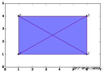
graph2 = buildGraph(raw_data=data, epsilon=7) #epsilon = 9 will build a "maximal complex"
ripsComplex2 = ripsFiltration(graph2, k=3)
SimplicialComplex.drawComplex(origData=data, ripsComplex=ripsComplex2[0], axes=[0,7,0,5])
[[{0},
  {1},
  {2},
  {3},
  {0, 1},
  {2, 3},
  {1, 2},
  {0, 3},
  {0, 2},
  {1, 3},
  {0, 1, 2},
  {0, 1, 3},
  {0, 2, 3},
  {1, 2, 3},
  {0, 1, 2, 3}],
 [0,
  0,
  0,
  0,
  3.0,
  3.0,
  5.0,
  5.0,
  5.8309518948453007,
  5.8309518948453007,
  5.8309518948453007,
  5.8309518948453007,
  5.8309518948453007,
  5.8309518948453007,
  5.8309518948453007]]
#return the n-simplices and weights in a complex
def nSimplices(n, filterComplex):
    nchain = []
    nfilters = []
    for i in range(len(filterComplex[0])):
        simplex = filterComplex[0][i]
        if len(simplex) == (n+1):
            nchain.append(simplex)
            nfilters.append(filterComplex[1][i])
    if (nchain == []): nchain = [0]
    return nchain, nfilters

#check if simplex is a face of another simplex
def checkFace(face, simplex):
    if simplex == 0:
        return 1
    elif (set(face) < set(simplex) and ( len(face) == (len(simplex)-1) )): #if face is a (n-1) subset of simplex
        return 1
    else:
        return 0
#build boundary matrix for dimension n ---> (n-1) = p
def filterBoundaryMatrix(filterComplex):
    bmatrix = np.zeros((len(filterComplex[0]),len(filterComplex[0])), dtype='>i8')
    #bmatrix[0,:] = 0 #add "zero-th" dimension as first row/column, makes algorithm easier later on
    #bmatrix[:,0] = 0
    i = 0
    for colSimplex in filterComplex[0]:
        j = 0
        for rowSimplex in filterComplex[0]:
            bmatrix[j,i] = checkFace(rowSimplex, colSimplex)
            j += 1
        i += 1
    return bmatrix
array([[0, 0, 0, 0, 1, 0, 0, 1, 1, 0, 0, 0, 0, 0, 0],
       [0, 0, 0, 0, 1, 0, 1, 0, 0, 1, 0, 0, 0, 0, 0],
       [0, 0, 0, 0, 0, 1, 1, 0, 1, 0, 0, 0, 0, 0, 0],
       [0, 0, 0, 0, 0, 1, 0, 1, 0, 1, 0, 0, 0, 0, 0],
       [0, 0, 0, 0, 0, 0, 0, 0, 0, 0, 1, 1, 0, 0, 0],
       [0, 0, 0, 0, 0, 0, 0, 0, 0, 0, 0, 0, 1, 1, 0],
       [0, 0, 0, 0, 0, 0, 0, 0, 0, 0, 1, 0, 0, 1, 0],
       [0, 0, 0, 0, 0, 0, 0, 0, 0, 0, 0, 1, 1, 0, 0],
       [0, 0, 0, 0, 0, 0, 0, 0, 0, 0, 1, 0, 1, 0, 0],
       [0, 0, 0, 0, 0, 0, 0, 0, 0, 0, 0, 1, 0, 1, 0],
       [0, 0, 0, 0, 0, 0, 0, 0, 0, 0, 0, 0, 0, 0, 1],
       [0, 0, 0, 0, 0, 0, 0, 0, 0, 0, 0, 0, 0, 0, 1],
       [0, 0, 0, 0, 0, 0, 0, 0, 0, 0, 0, 0, 0, 0, 1],
       [0, 0, 0, 0, 0, 0, 0, 0, 0, 0, 0, 0, 0, 0, 1],
       [0, 0, 0, 0, 0, 0, 0, 0, 0, 0, 0, 0, 0, 0, 0]])
下面的函数是用来减化前面描述的边界矩阵 (当我们手工计算的时候)。
#returns row index of lowest "1" in a column i in the boundary matrix
def low(i, matrix):
    col = matrix[:,i]
    col_len = len(col)
    for i in range( (col_len-1) , -1, -1): #loop through column from bottom until you find the first 1
        if col[i] == 1: return i
    return -1 #if no lowest 1 (e.g. column of all zeros), return -1 to be 'undefined'

#checks if the boundary matrix is fully reduced
def isReduced(matrix):
    for j in range(matrix.shape[1]): #iterate through columns
        for i in range(j): #iterate through columns before column j
            low_j = low(j, matrix)
            low_i = low(i, matrix)
            if (low_j == low_i and low_j != -1):
                return i,j #return column i to add to column j
    return [0,0]

#the main function to iteratively reduce the boundary matrix
def reduceBoundaryMatrix(matrix):
    #this refers to column index in the boundary matrix
    reduced_matrix = matrix.copy()
    matrix_shape = reduced_matrix.shape
    memory = np.identity(matrix_shape[1], dtype='>i8') #this matrix will store the column additions we make
    r = isReduced(reduced_matrix)
    while (r != [0,0]):
        i = r[0]
        j = r[1]
        col_j = reduced_matrix[:,j]
        col_i = reduced_matrix[:,i]
        #print("Mod: add col %s to %s \n" % (i+1,j+1)) #Uncomment to see what mods are made
        reduced_matrix[:,j] = np.bitwise_xor(col_i,col_j) #add column i to j
        memory[i,j] = 1
        r = isReduced(reduced_matrix)
    return reduced_matrix, memory
Mod: add col 6 to 8

Mod: add col 7 to 8

Mod: add col 5 to 8

Mod: add col 7 to 9

Mod: add col 5 to 9

Mod: add col 6 to 10

Mod: add col 7 to 10

Mod: add col 11 to 13

Mod: add col 12 to 14

Mod: add col 13 to 14
(array([[0, 0, 0, 0, 1, 0, 0, 0, 0, 0, 0, 0, 0, 0, 0],
        [0, 0, 0, 0, 1, 0, 1, 0, 0, 0, 0, 0, 0, 0, 0],
        [0, 0, 0, 0, 0, 1, 1, 0, 0, 0, 0, 0, 0, 0, 0],
        [0, 0, 0, 0, 0, 1, 0, 0, 0, 0, 0, 0, 0, 0, 0],
        [0, 0, 0, 0, 0, 0, 0, 0, 0, 0, 1, 1, 1, 0, 0],
        [0, 0, 0, 0, 0, 0, 0, 0, 0, 0, 0, 0, 1, 0, 0],
        [0, 0, 0, 0, 0, 0, 0, 0, 0, 0, 1, 0, 1, 0, 0],
        [0, 0, 0, 0, 0, 0, 0, 0, 0, 0, 0, 1, 1, 0, 0],
        [0, 0, 0, 0, 0, 0, 0, 0, 0, 0, 1, 0, 0, 0, 0],
        [0, 0, 0, 0, 0, 0, 0, 0, 0, 0, 0, 1, 0, 0, 0],
        [0, 0, 0, 0, 0, 0, 0, 0, 0, 0, 0, 0, 0, 0, 1],
        [0, 0, 0, 0, 0, 0, 0, 0, 0, 0, 0, 0, 0, 0, 1],
        [0, 0, 0, 0, 0, 0, 0, 0, 0, 0, 0, 0, 0, 0, 1],
        [0, 0, 0, 0, 0, 0, 0, 0, 0, 0, 0, 0, 0, 0, 1],
        [0, 0, 0, 0, 0, 0, 0, 0, 0, 0, 0, 0, 0, 0, 0]]),
 array([[1, 0, 0, 0, 0, 0, 0, 0, 0, 0, 0, 0, 0, 0, 0],
        [0, 1, 0, 0, 0, 0, 0, 0, 0, 0, 0, 0, 0, 0, 0],
        [0, 0, 1, 0, 0, 0, 0, 0, 0, 0, 0, 0, 0, 0, 0],
        [0, 0, 0, 1, 0, 0, 0, 0, 0, 0, 0, 0, 0, 0, 0],
        [0, 0, 0, 0, 1, 0, 0, 1, 1, 0, 0, 0, 0, 0, 0],
        [0, 0, 0, 0, 0, 1, 0, 1, 0, 1, 0, 0, 0, 0, 0],
        [0, 0, 0, 0, 0, 0, 1, 1, 1, 1, 0, 0, 0, 0, 0],
        [0, 0, 0, 0, 0, 0, 0, 1, 0, 0, 0, 0, 0, 0, 0],
        [0, 0, 0, 0, 0, 0, 0, 0, 1, 0, 0, 0, 0, 0, 0],
        [0, 0, 0, 0, 0, 0, 0, 0, 0, 1, 0, 0, 0, 0, 0],
        [0, 0, 0, 0, 0, 0, 0, 0, 0, 0, 1, 0, 1, 0, 0],
        [0, 0, 0, 0, 0, 0, 0, 0, 0, 0, 0, 1, 0, 1, 0],
        [0, 0, 0, 0, 0, 0, 0, 0, 0, 0, 0, 0, 1, 1, 0],
        [0, 0, 0, 0, 0, 0, 0, 0, 0, 0, 0, 0, 0, 1, 0],
        [0, 0, 0, 0, 0, 0, 0, 0, 0, 0, 0, 0, 0, 0, 1]]))
所以 reduceBoundaryMatrix 方法返回两个矩阵,减化边界矩阵和记录简化算法所有动作的记忆矩阵。这是必要的,所以我们可以查一下边界矩阵的每一列实际上指的是什么。它减少了边界矩阵中的每一列并不一定是一个单形,可能是一组单形,如某个 \(n\) 维的环。
下面的函数使用减化的矩阵来读取所有在滤流中特征生成和消亡的间隔。
def readIntervals(reduced_matrix, filterValues): #reduced_matrix includes the reduced boundary matrix AND the memory matrix
    #store intervals as a list of 2-element lists, e.g. [2,4] = start at "time" point 2, end at "time" point 4
    #note the "time" points are actually just the simplex index number for now. we will convert to epsilon value later
    intervals = []
    #loop through each column j
    #if low(j) = -1 (undefined, all zeros) then j signifies the birth of a new feature j
    #if low(j) = i (defined), then j signifies the death of feature i
    for j in range(reduced_matrix[0].shape[1]): #for each column (its a square matrix so doesn't matter...)
        low_j = low(j, reduced_matrix[0])
        if low_j == -1:
            interval_start = [j, -1]
            intervals.append(interval_start) # -1 is a temporary placeholder until we update with death time
            #if no death time, then -1 signifies feature has no end (start -> infinity)
            #-1 turns out to be very useful because in python if we access the list x[-1] then that will return the
            #last element in that list. in effect if we leave the end point of an interval to be -1
            # then we're saying the feature lasts until the very end
        else: #death of feature
            feature = intervals.index([low_j, -1]) #find the feature [start,end] so we can update the end point
            intervals[feature][1] = j #j is the death point
            #if the interval start point and end point are the same, then this feature begins and dies instantly
            #so it is a useless interval and we dont want to waste memory keeping it
            epsilon_start = filterValues[intervals[feature][0]]
            epsilon_end = filterValues[j]
            if epsilon_start == epsilon_end: intervals.remove(intervals[feature])
    return intervals

def readPersistence(intervals, filterComplex):
    #this converts intervals into epsilon format and figures out which homology group each interval belongs to
    persistence = []
    for interval in intervals:
        start = interval[0]
        end = interval[1]
        homology_group = (len(filterComplex[0][start]) - 1) #filterComplex is a list of lists [complex, filter values]
        epsilon_start = filterComplex[1][start]
        epsilon_end = filterComplex[1][end]
        persistence.append([homology_group, [epsilon_start, epsilon_end]])
    return persistence
这些都是特征出现和消亡的间隔。readPersistence 函数只会将边界矩阵目录的起始 / 结束点转换成相应的 \(\epsilon\) 值。它也会计算出每个区间所属的同调群 (即是哪个连通数维度)。
[[0, [0, 5.8309518948453007]],
 [0, [0, 3.0]],
 [0, [0, 5.0]],
 [0, [0, 3.0]],
 [1, [5.0, 5.8309518948453007]]]
这个函数只会为单个维度绘制持续条码图。
import matplotlib.pyplot as plt
def graph_barcode(persistence, homology_group = 0):
    #this function just produces the barcode graph for each homology group
    xstart = [s[1][0] for s in persistence if s[0] == homology_group]
    xstop = [s[1][1] for s in persistence if s[0] == homology_group]
    y = [0.1 * x + 0.1 for x in range(len(xstart))]
    plt.hlines(y, xstart, xstop, color='b', lw=4)
    #Setup the plot
    ax = plt.gca()
    plt.ylim(0,max(y)+0.1)
    ax.yaxis.set_major_formatter(plt.NullFormatter())
    plt.xlabel('epsilon')
    plt.ylabel("Betti dim %s" % (homology_group,))
plt.show()
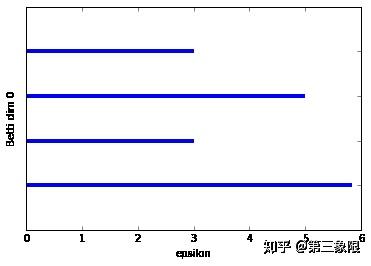
太爽了,终于是持续同调的完整实现。
我们已经画出了前两个连通数的条码图。第一个条形码图比较稀松平常,因为我们想看到的是一些比其他的长得多的条,那才能说明真正的特征。在这种情况下,连通维度 \(0\) 的条码图有最长的条,它代表着形成盒子的单连通组件,但它并没有比第二长的条长很多。这主要是示例非常简单的特征。如果我再加几个点,我们就会发现一个更长的最长条。
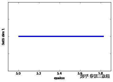
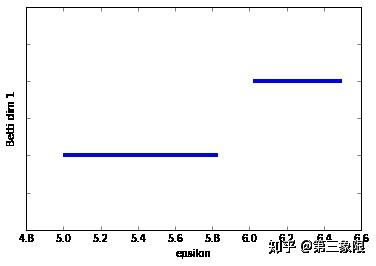
连通维度 \(2\) 的条码图的形状就要好得多。我们明显只有一个长条,这表明 \(1\) 维的环会一直存在到 \(\epsilon =5.8\) 时盒子被 “填充” 的时候。
持续同调非常重要的特征是能够找到一些有有趣拓扑特征的数据点。如果所有持续同调能够给我们条码图,并告诉我们有多少连接组件和环,那它将非常有用,但也有所不足。
我们真正想做的是说,“看,条形码图展示了这有一个有统计学意义的 \(1\) 维环,我想知道那些数据点形成了这个环?”
为了来测试这个过程,我们来稍微修改一下这个简单的 “盒子” 的单纯复形,并加入另一条边(给我们另一个连接组件)。
graph2b = buildGraph(raw_data=data_b, epsilon=8) #epsilon is set to a high value to create a maximal complex
rips2b = ripsFiltration(graph2b, k=3)
SimplicialComplex.drawComplex(origData=data_b, ripsComplex=rips2b[0], axes=[0,14,0,6])
随着我们将 \(\epsilon\) 设成一个较高值,这形成了最大的复形。但我试着设计数据使得 “真实” 的特征是一个盒子( \(1\) 维的环),以及右边的一条边,总共两个 “真正的” 连接组件。
那让我们在数据上进行持续同调。
bm2b = filterBoundaryMatrix(rips2b)
rbm2b = reduceBoundaryMatrix(bm2b)
intervals2b = readIntervals(rbm2b, rips2b[1])
persist2b = readPersistence(intervals2b, rips2b)
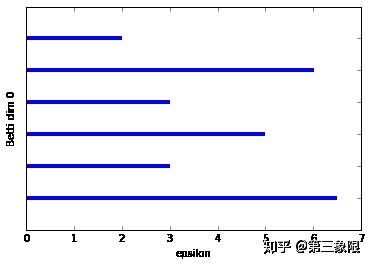
我们可以看到在 \(0\) 维连通数中两个连接组件(最长的两条横杠),还有 \(1\) 维连通数中的两个条,但一个很明显是另一个的两倍长。较短的条来自右侧边线和左侧盒子最左的两条线形成的环。
因此,在这一点上,我们认为我们有一个重要的 \(1\) 维环,但我们不知道哪些点形成这个环,因此,如果我们愿意,我们可以进一步分析这些数据的子集。
为了把它表示出来,我们只需要用到我们的归约算法返回给我们的记忆矩阵。首先,我们从 intervals2b 列表找到我们需要的区间,在例子中,它是第一个元素,然后我们得到起始点(因为这表明了特性的诞生)。起始点是边界数组中的一个索引值,所以我们将在记忆数组中找到那一列并在那一列中找到带 1 的单元。在该列中带 1 的行是群中的其他单形(包括列本身)。
[[0, [0, 6.5]],
 [0, [0, 3.0]],
 [0, [0, 5.0]],
 [0, [0, 3.0]],
 [0, [0, 6.0207972893961479]],
 [0, [0, 2.0]],
 [1, [5.0, 5.8309518948453007]],
 [1, [6.0207972893961479, 6.5]]]
首先,看看同调群 1 的区间,然后我们想要 \(\epsilon\) 范围是从 \(5.0\) 到 \(5.83\) 的区间。那是在持续性列表的索引 \(6\) ,也是间隔列表的索引 \(6\) 。间隔列表,不是 \(\epsilon\) 的起始和终点,有索引值,因此我们可以在记忆矩阵中检索到单形。
所以这是记忆矩阵索引值 = \(10\) 的列。所以我们自然而然地知道无论索引 \(10\) 中的单形是什么,都是环的一部分,也是这一列中有 \(1\) 的行。
#so the simplices with indices 7,8,9,10 lie on our 1-dimensional cycle, let's find what those simplices are
rips2b[0][7:11] #range [start:stop], but stop is non-inclusive, so put 11 instead of 10
完全正确!这就是我们在条码中看到的 1 维循环的 \(1\) 维单形列表。从这个列表到原始数据点应该很简单,所以我不会在这里向你介绍这些细节。
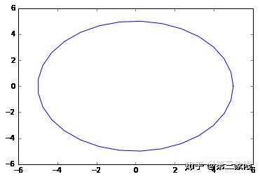
那让我们用一些更实际的数据来试试。我们将像之前做的那样,从圆中取一些数据。在这个例子中,我在 ripsFiltration 函数中设置参数 k=2,那么它最多只会生成 \(2\) 维单形。这只是为了减少内存的需要。如果你有一台有很多内存的电脑,你当然可以把 k 设置成 \(3\) ,但我不会让它更大。通常我们对连接的分量和 1 或者 \(2\) 维环感兴趣。拓扑特征在维度上的效用貌似是逐渐递减的,并且内存和算法运行时间的代价一般不太值得。
注意:接下来可能需要一段时间运行,大概要几分钟。这是因为在这些教程中编写的代码是为了清晰和方便而进行的优化,而不是为了效率和速度。如果我们想要在任何地方接近一个现成的 TDA 库,那么有很多性能可以优化并且应该被制造。我计划到时候写一篇后续文章,讨论最合理的算法和数据结构优化,因为我希望在未来开发一个合理高效的 python 开源 TDA 库,希望能得到一些帮助。
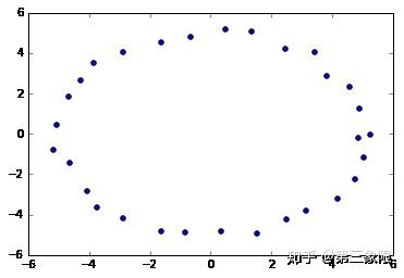
n = 30 #number of points to generate
#generate space of parameter
theta = np.linspace(0, 2.0*np.pi, n)
a, b, r = 0.0, 0.0, 5.0
x = a + r*np.cos(theta)
y = b + r*np.sin(theta)
#code to plot the circle for visualization
plt.plot(x, y)
plt.show()
xc = np.random.uniform(-0.25,0.25,n) + x #add some "jitteriness" to the points (but less than before, reduces memory)
yc = np.random.uniform(-0.25,0.25,n) + y
fig, ax = plt.subplots()
ax.scatter(xc,yc)
plt.show()
circleData = np.array(list(zip(xc,yc)))
graph4 = buildGraph(raw_data=circleData, epsilon=3.0)
rips4 = ripsFiltration(graph4, k=2)
SimplicialComplex.drawComplex(origData=circleData, ripsComplex=rips4[0], axes=[-6,6,-6,6])
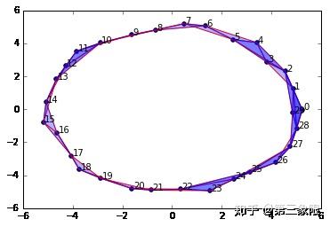
显然,持续同调告诉我们,我们有 \(1\) 个连接组件和 \(1\) 维环。
len(rips4[0])
#On my laptop, a rips filtration with more than about 250 simplices will take >10 mins to compute persistent homology
#anything < ~220 only takes a few minutes or less
%%time
bm4 = filterBoundaryMatrix(rips4)
rbm4 = reduceBoundaryMatrix(bm4)
intervals4 = readIntervals(rbm4, rips4[1])
persist4 = readPersistence(intervals4, rips4)
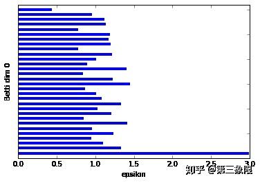
我们可以清楚地看到,在 Betti dim 0 条码图中,有一个明显较长的条,这表明我们只有一个明显的连接组件。这很符合我们绘制的圆形数据。
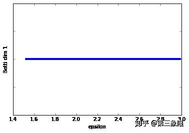
Betti dim 1 条码图更简单,因为它只有一个条,所以我们当然有明显的特征,即 \(1\) 维循环。
那么,像之前一样,我们开始测试我们的算法。
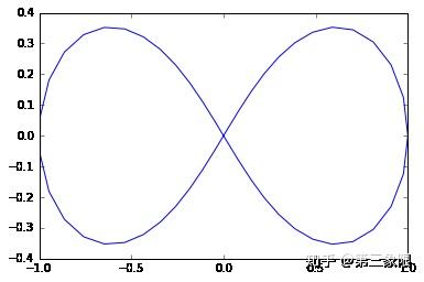
我准备从一个叫双扭线(也可以叫 \(8\) 字形)的图形中采样。正如你所见,它应该有一个连接组件和两个 \(1\) 维环。
n = 50
t = np.linspace(0, 2*np.pi, num=n)
#equations for lemniscate
x = np.cos(t) / (np.sin(t)**2 + 1)
y = np.cos(t) * np.sin(t) / (np.sin(t)**2 + 1)

plt.plot(x, y)
plt.show()
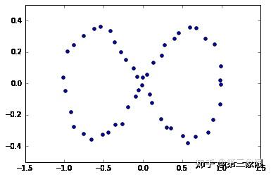
x2 = np.random.uniform(-0.03, 0.03, n) + x #add some "jitteriness" to the points
y2 = np.random.uniform(-0.03, 0.03, n) + y
fig, ax = plt.subplots()
ax.scatter(x2,y2)
plt.show()
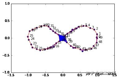
graph5 = buildGraph(raw_data=figure8Data, epsilon=0.2)
rips5 = ripsFiltration(graph5, k=2)
SimplicialComplex.drawComplex(origData=figure8Data, ripsComplex=rips5[0], axes=[-1.5,1.5,-1, 1])
%%time
bm5 = filterBoundaryMatrix(rips5)
rbm5 = reduceBoundaryMatrix(bm5)
intervals5 = readIntervals(rbm5, rips5[1])
persist5 = readPersistence(intervals5, rips5)
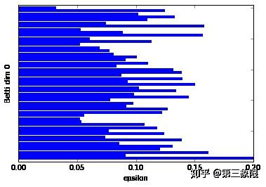
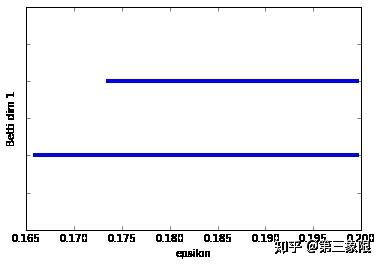
正如我们所想,Betti dim 0 显示有一个条明显长于其他,Betti dim 1 显示有两个条,即有两个 \(1\) 维环。
结束
第 5 章是关于持续同调的子系列的最后一章。现在,你应该具备理解和使用现有的持续同调工具所需的所有知识,甚至可以自己构建自己的工具。