Training Dynamics
Learning Rate Schedules
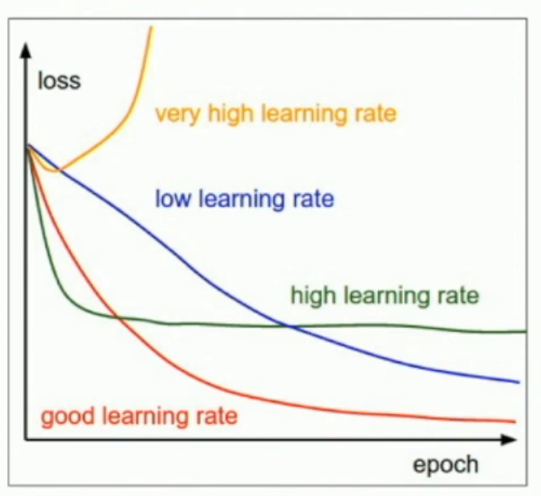
很多时候,我们既希望快速让 loss 下降,也希望能让 loss 降到尽量低。因此,我们往往会在学习的时候改变 learning rate。而改变学习率的方法,称为 learning rate schedule。
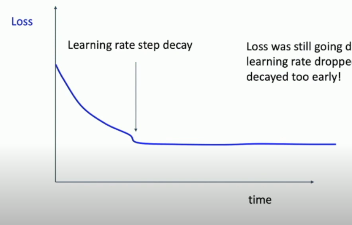
Step Decay
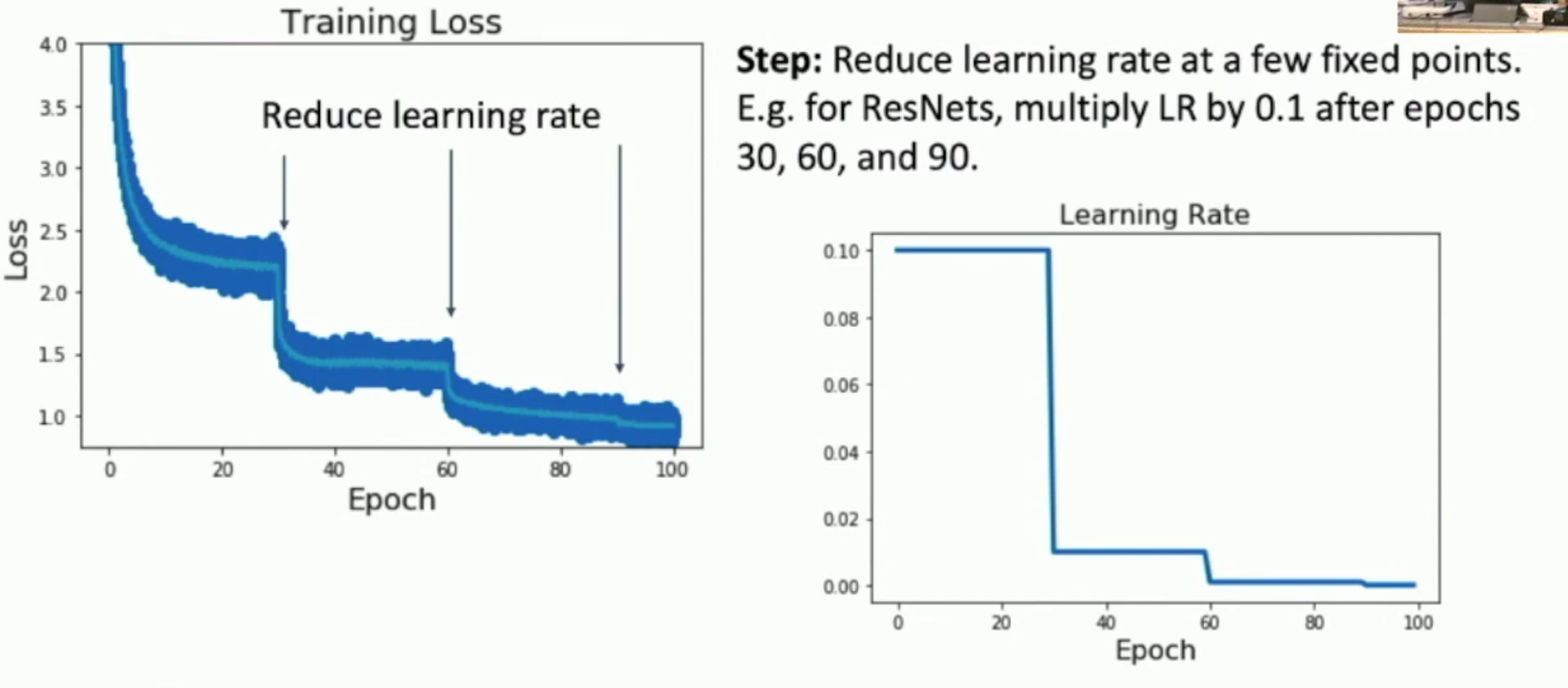
如图,每隔一段时间,就会进行学习率下降。从而保证我们一直处于 high learning rate 的左侧的“快速下降区”。
但是,这种方法的坏处是:hyperparameter 过于多。你需要调整
- initial learning rate
- decay rate
- decay interval
- 当然,也有一种 heuristic 的方法来 tuning:先训练,再找 loss plateau,然后在 plateau 的起始处进行 decay
因此,tuning can be a little tricky.
Cosine Decay
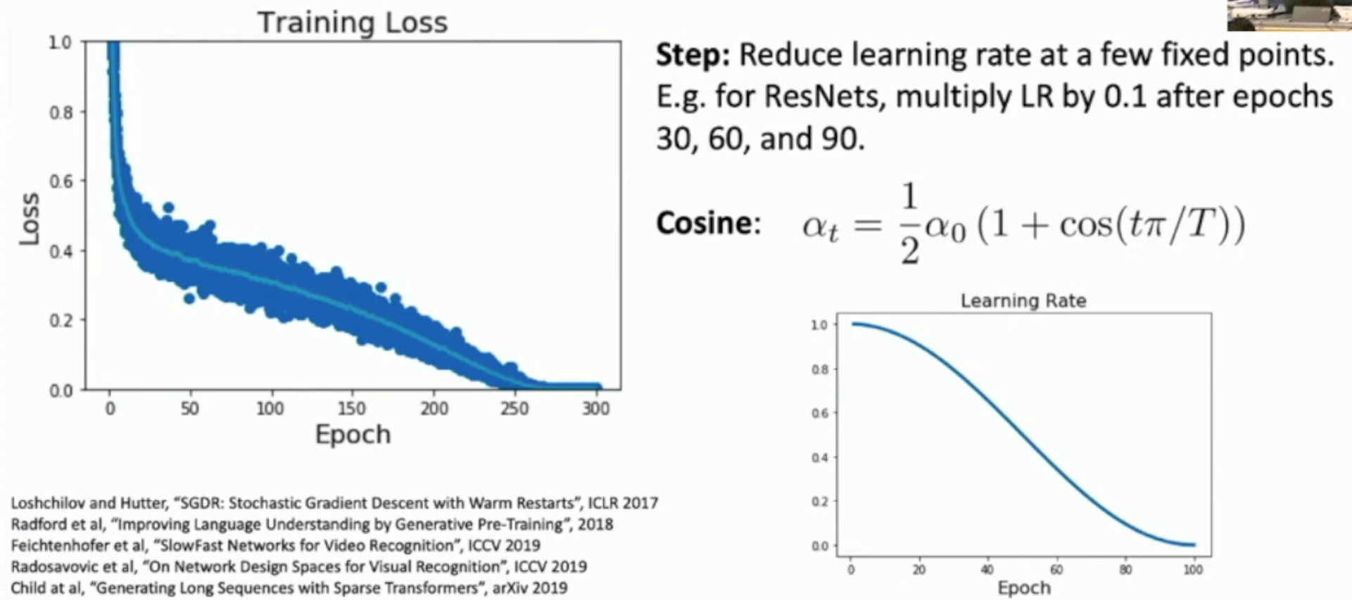
好处:只要给定 initial learning rate 和 end learning rate,就可以自动得到一个 learning rate 与 epoch 的对应关系。
同样地还有:
- Linear decay: \(a_t = a_0 t / T\)
- Inverse square root decay: \(a_t = a_0 / \sqrt{t}\)
- And ..., just constant decay: \(a_t = a_0\)
Rule of Thumb
- 不要在一开始就调整 learning schedule,这应该是最后做的事
- 一开始请直接使用 constant schedule
- 对于 SGD+Momentum,有一个 non-trivial decay schedule 可能是好事。但是对于更复杂的 optimizers (e.g. Adam),其实没必要使用这些 fancy schedules - constant schedule is okay.
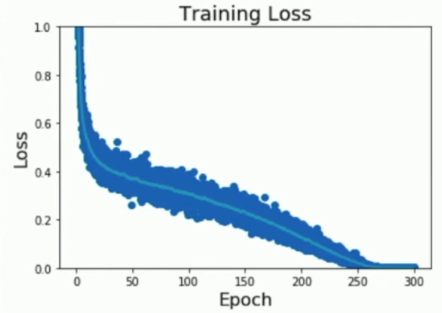
Sidenote: Plotting losses like the image below (i.e. average training loss as well as the variance) helps you debug your code.
Sidenote: Early Stopping
在训练的时候,我们需要一直关注以下两张图:
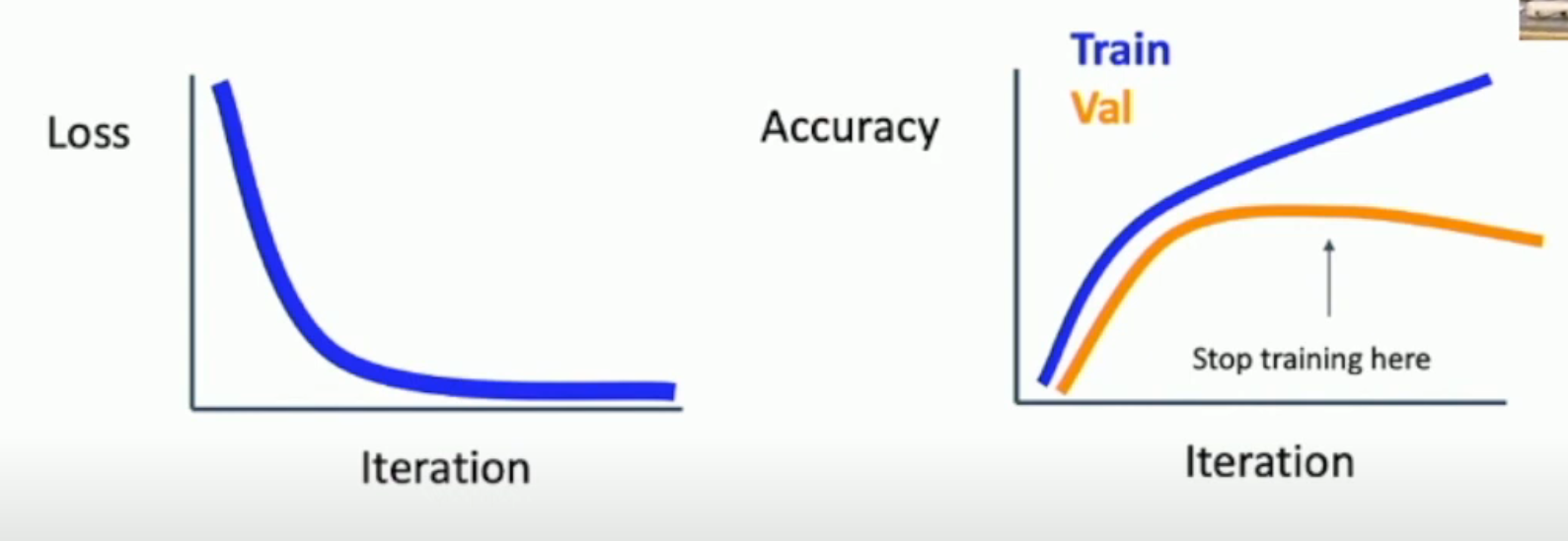
从而,我们可以在 validation accuracy 下降的时候,及时停止 training。
Hyperparameter Optimization
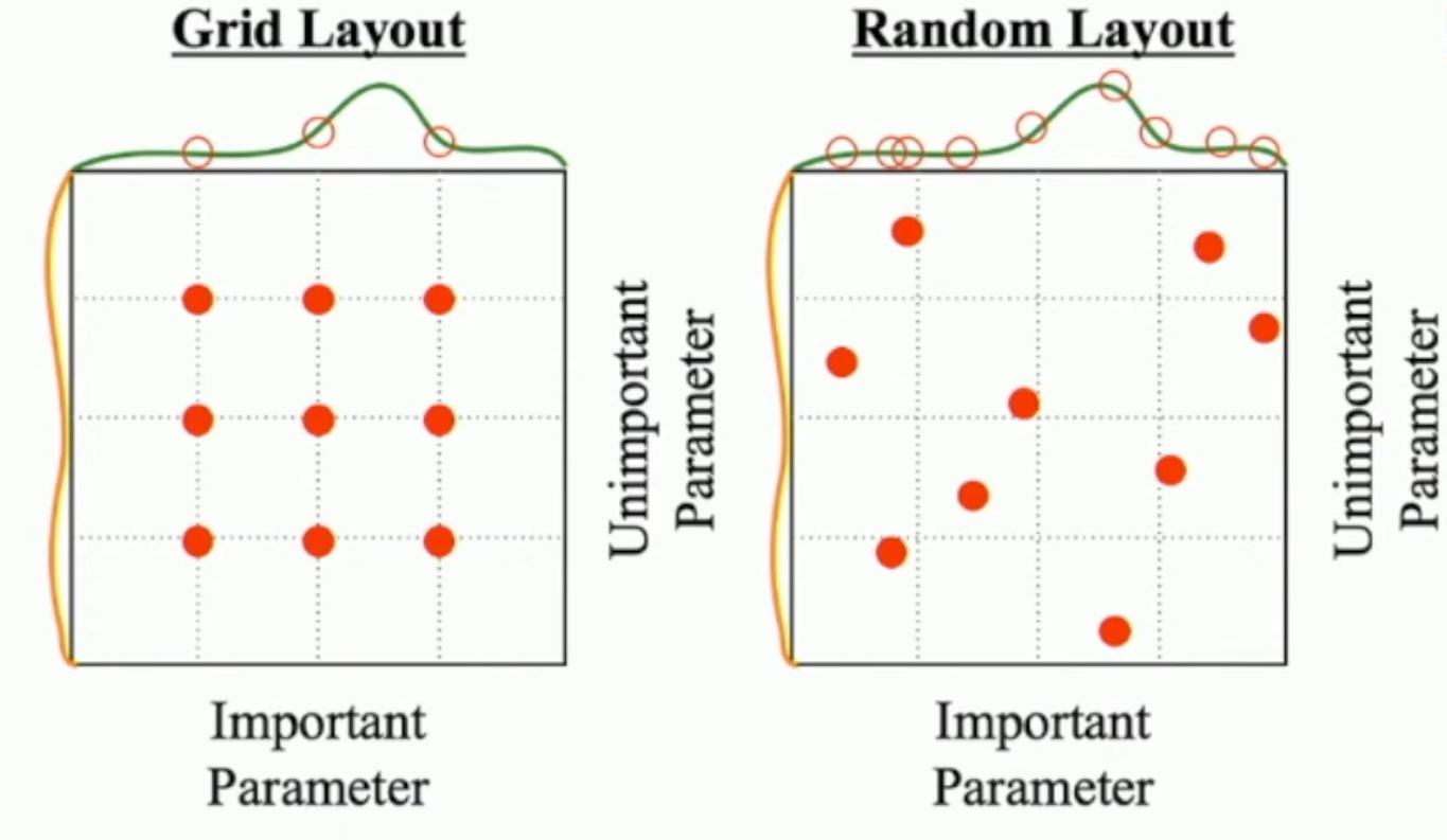
一种方法,就是 grid search;另一种方法,就是 random search (in some interval)。
Random search 的好处:
- 在 hyperparameter 数量很多的时候,极大地降低计算量
- 对于存在部分 unimportant parameters 的情况,我们随机取点(如右图),可以避免左侧的重复计算
很多时候,hyperparameter 之间其实是相关的,如下图所示:
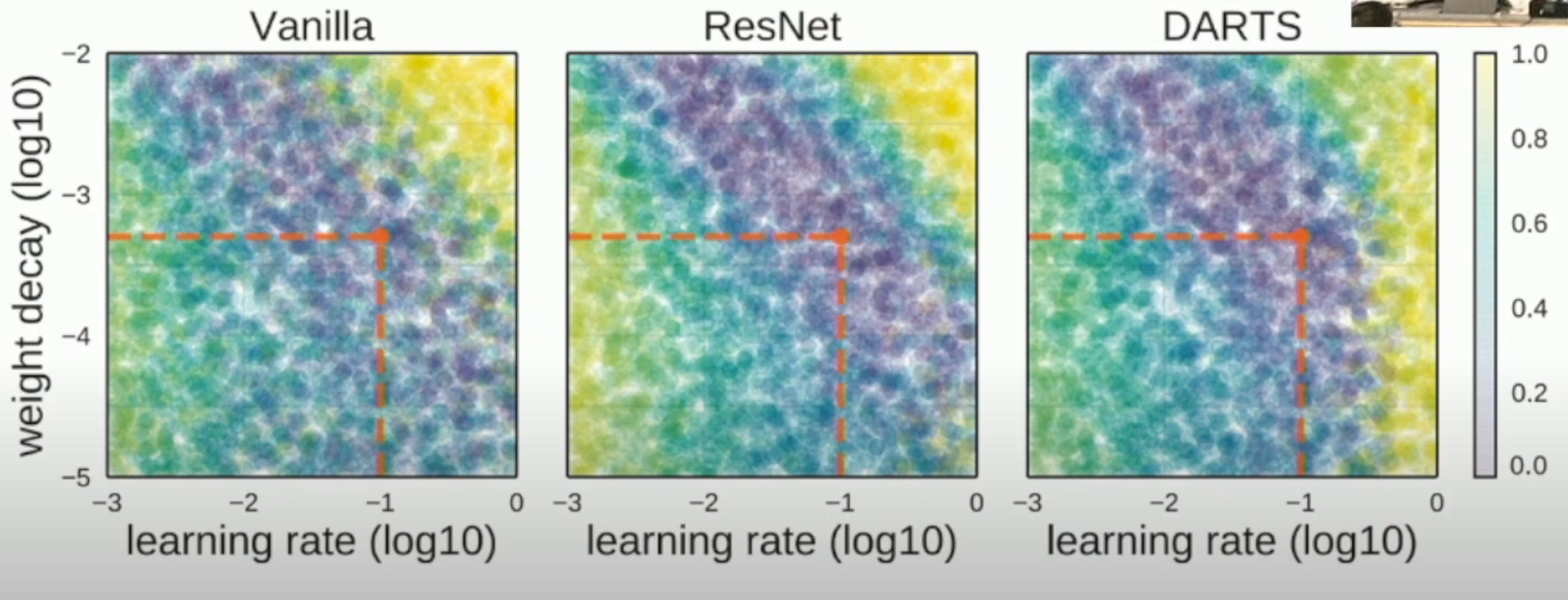
因此,grid/random search 是有必要的。你不能假设 hyperparameters 之间独立,然后每一次只调一个 hyperparameter。你必须一起调整。
另外,我们甚至可以对 hyperparameter 求梯度,从而实现所谓 hyper gradient descent。当然,这种做法并不 popular,因为计算成本太高。
How To Choose Hyperparameters
Step 1: Check initial loss without any weight decay
- 因为我们可以解析地计算出最开始的 loss 的期望值大概是多少。因此,这可以作为一开始的 sanity check,用于 debug
Step 2: Overfit a small sample
- 进一步 debug
- 因为 small sample 可以瞬间训练完,因此,这一步中,你还可以 interactively 选择合适的 learning rate(范围)、architecture、optimizer, initialization 等等
- i.e. 保证 architecture, optimizer, learning rate, initialization etc 适合你的 data
- 这一步确定下来了 architecture, optimizer, initialization,以及 learning rate 大致的范围
Step 3: Tune the learning rate
- Use the architecture from the previous step, use all training data, turn on small weight decay, find a learning rate that makes the lossdrop significantly within ~100 iterations
- Good learning rates to try:1e-1,1e-2,1e-3,1e-4
- 这一步排除掉了一些不能用的 learning rate
Step 4: Coarse grid
- Choose a few values of learning rate and weight decay around whatworked from Step 3, train a few models for ~1-5 epochs.
- Good weight decay to try:1e-4,1e-5,0
- 这一步
Step 5: Refine grid, train longer
- Pick best models from Step 4, train them for longer (~10-20 epochs) without learning rate decay
Step 6: Look at learning curves
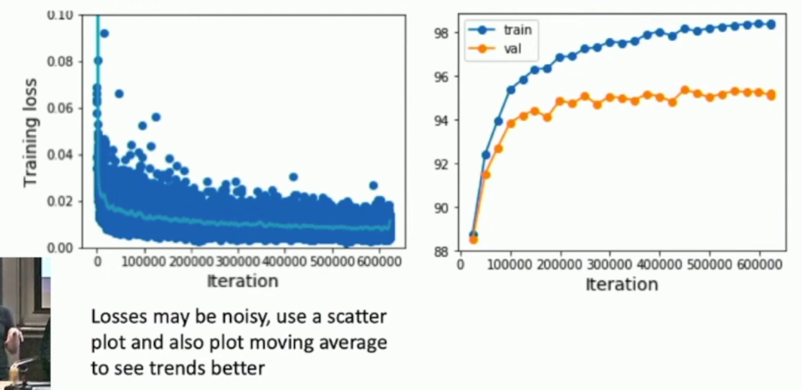
如图:
对于 loss graph 而言:
- 如果 loss 降得太慢,就说明 lr 太低了
- 如果 loss 一开始降得快,但是后来就不降了,就说明 lr 太高了,你需要 introduce some learning decay
- 如果你采用了 weight decay 的方法,但是却出现了如下的情况,那么就说明你 decay 得太早了
对于 validation and training accuracy 而言:
- 如果两者一直稳步上升,且之间有一定的 gap(直到训练结束还在上升),那么就说明你训练的轮数太少了
- 如果 training 上升,validation 下降,就是 overfitting
- 如果两者虽然在上升,但是两者之间得 gap 太小,就是 underfitting
- 目前没有好的理论解释。只能说 training 和 validation 之间有一条天然的“鸿沟”。
Step 7: Repeat Step 5, Until It's Paper Submission Deadline
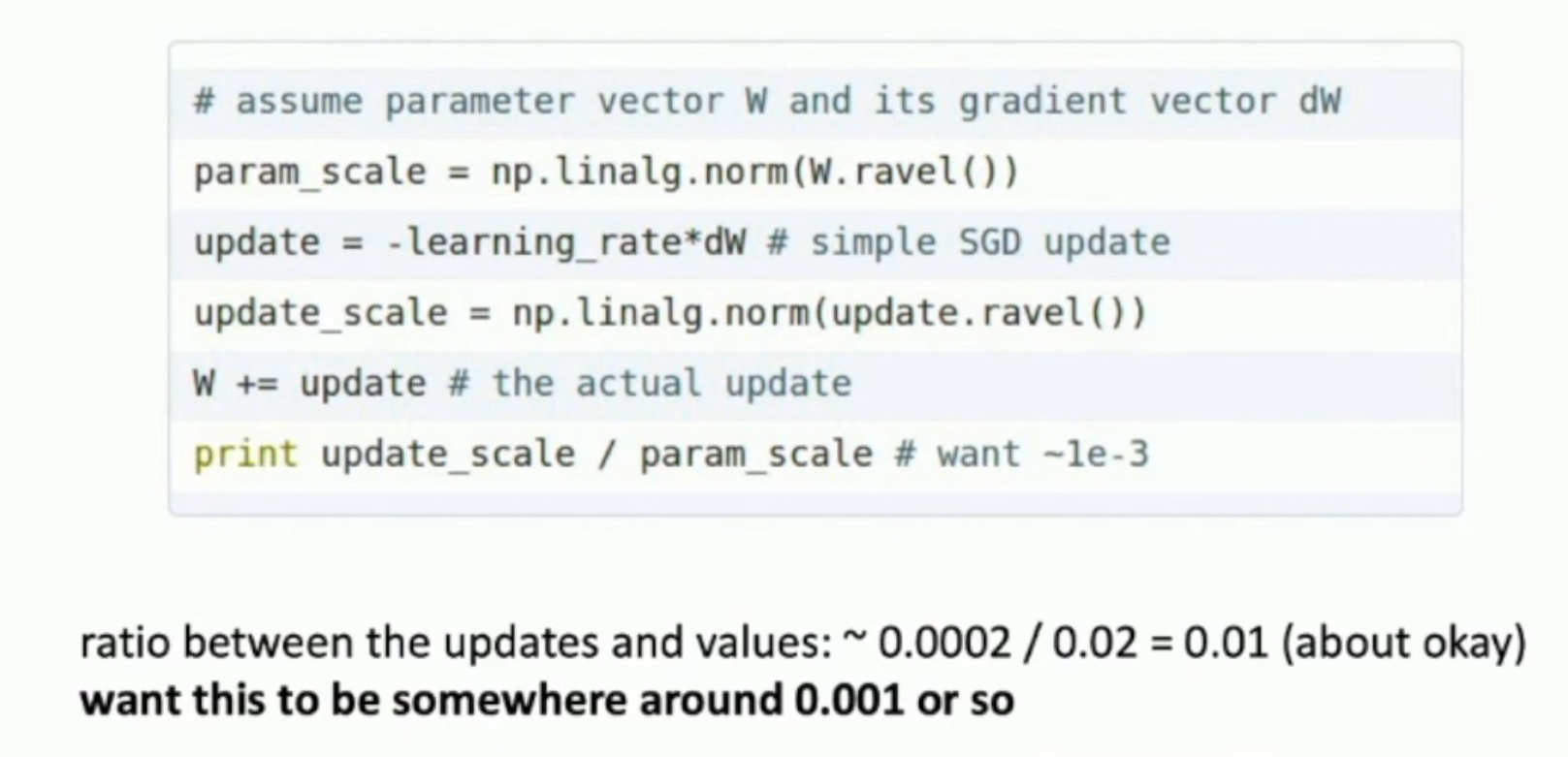
Sidenote: Track Ratio of Weight Update / Weight Magnitude
After Training
Model Ensembles
- Train multiple independent models
- At test time average their results (e.g. Take average of predicted probability distributions, then choose
argmax)
Normally, you can enjoy 2% extra performance via this method
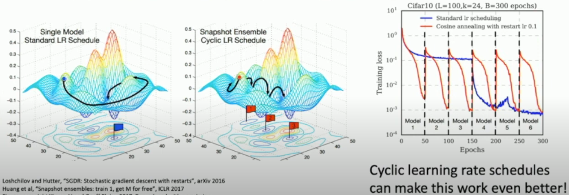
Multiple Snapshots
Instead of training independent models, use multiple snapshots of a single model during training!
Polyak Averaging
Instead of using actual parameter vector, keep a moving average of the parameter vector and use that at test time.
while True:
    data_batch = dataset.sample_data_batch()
    loss = network.forward(data_batch)
    dx = network.backward()
    x += - learning_rate * dx
    x_test = 0.995*x_test + 0.005*x # This is the "moving average" weight
    # that is use for test set
Transfer Learning
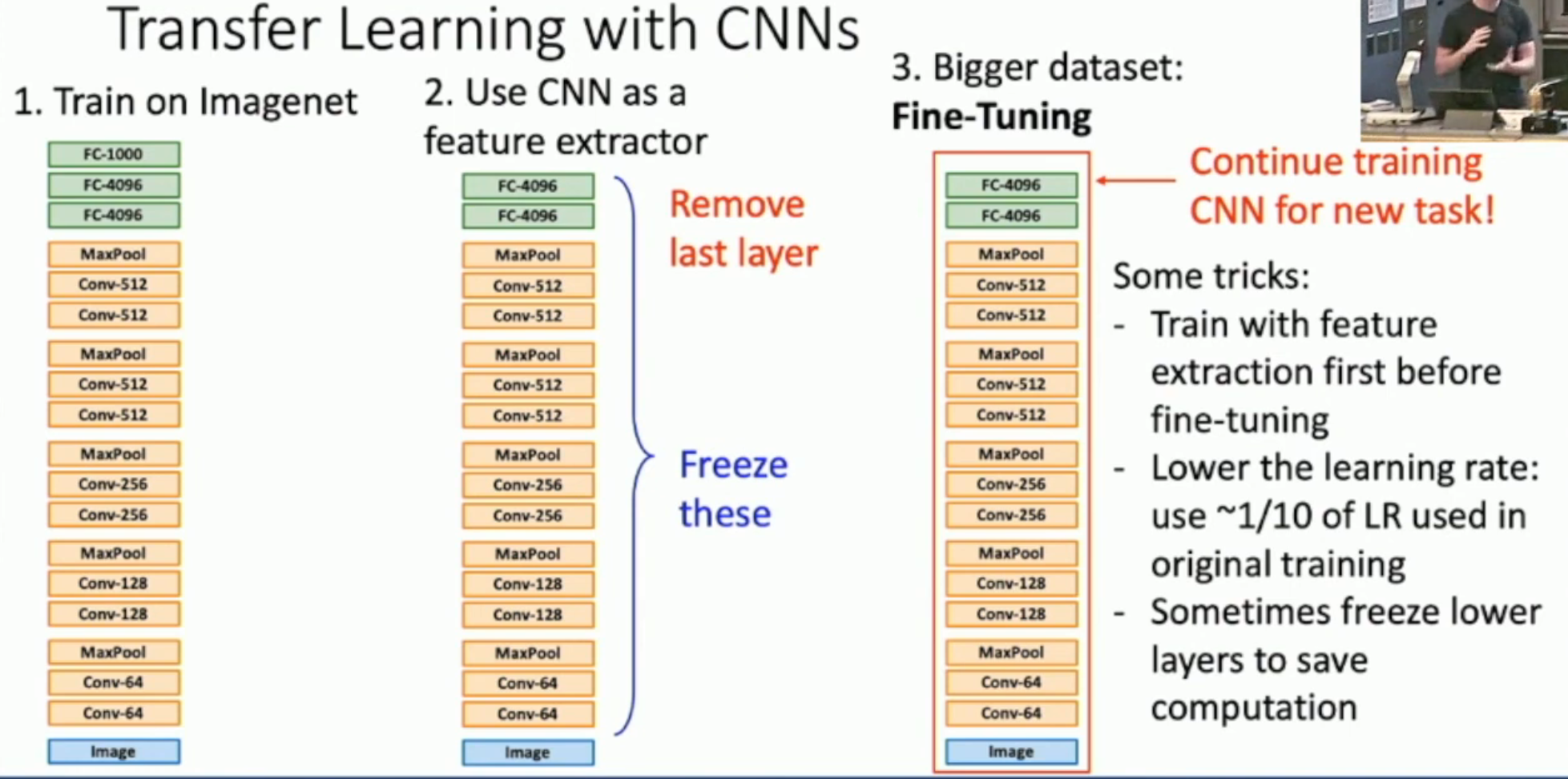
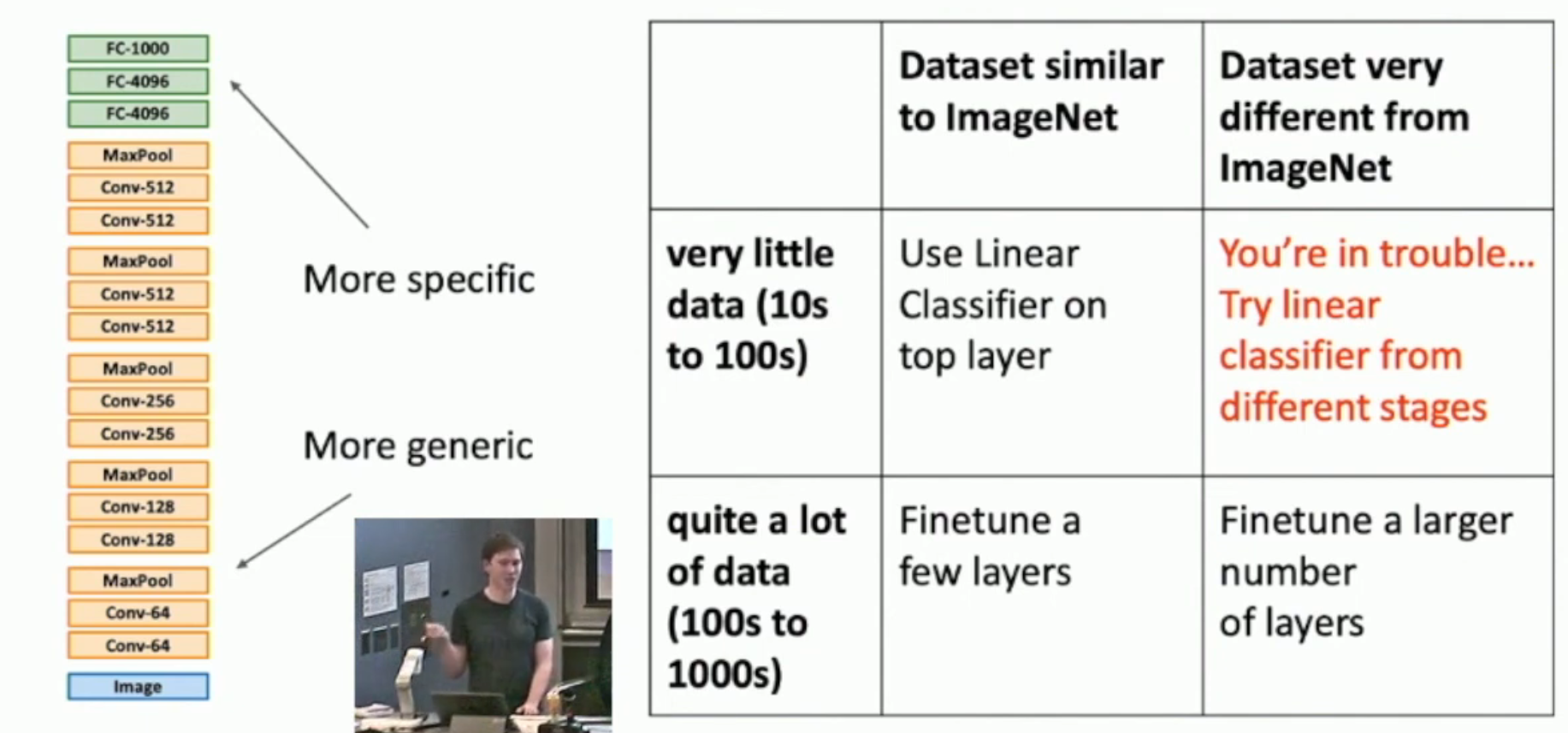
如图,
- 对于小样本,我们往往直接采用 feature extractor 的方式。就是冻结所有 feature extractor layers,然后只训练最后一层
- 对于大样本,我们可以微调整个模型。以下是几个 fine-tuning tricks
- training (with feature extraction) before tuning
- use lower learning rate
- remember, you are tuning on a pre-trained model, not training
- freeze lower layers (i.e. layers that extract more coarse-grained and common features) to save computation
总结:
Transfer Learning in Practice
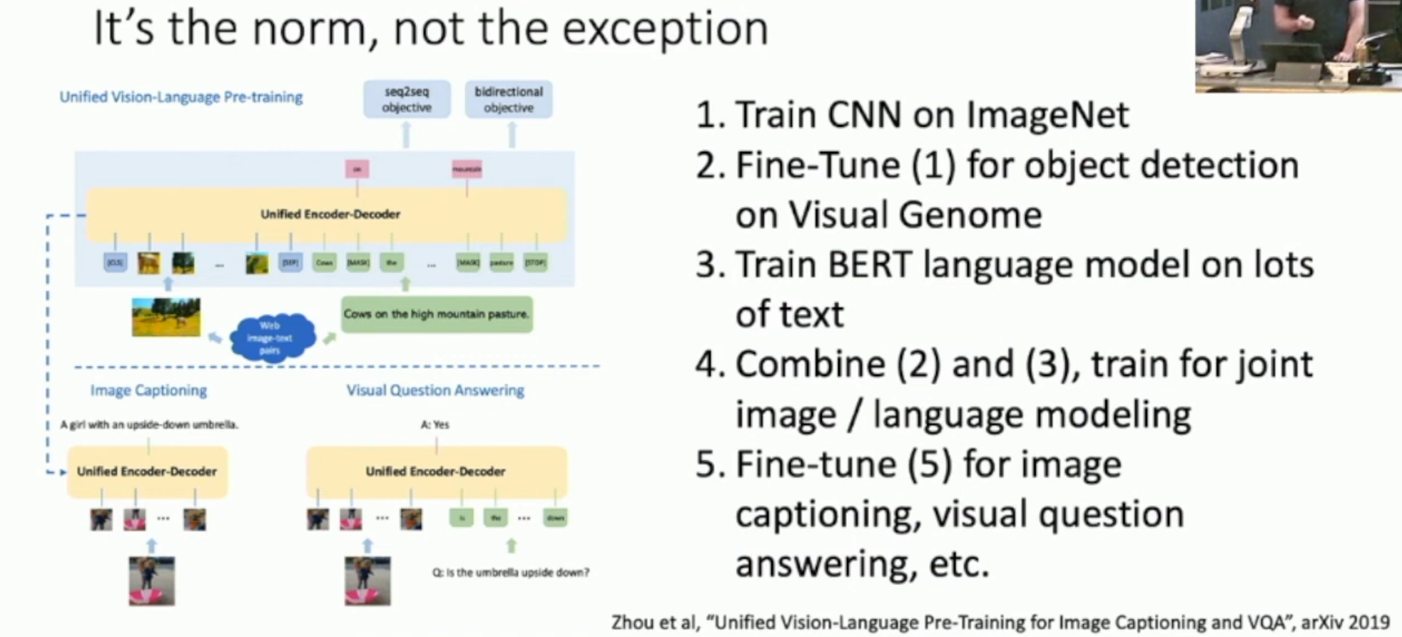
如上:我们先训练分类,再微调图形检测;同时训练一个 NLP 模型。然后把图形检测模型和 NLP 模型结合起来,训练 joint image / language modeling。最后再对目标任务,i.e. image captioning, visaual question answering 任务进行微调。
Is Pre-training a Must?
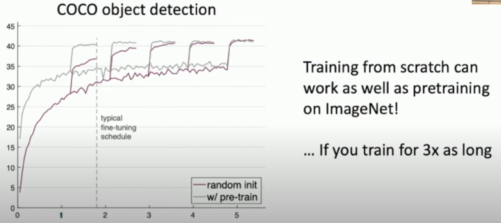
如图,对比“直接使用模型在 COCO 数据集上进行训练”和“使用(在其他数据集上)pre-trained model 在 COCO 上微调”,前者也可以赶上后者,但是要花很多时间(左图)。
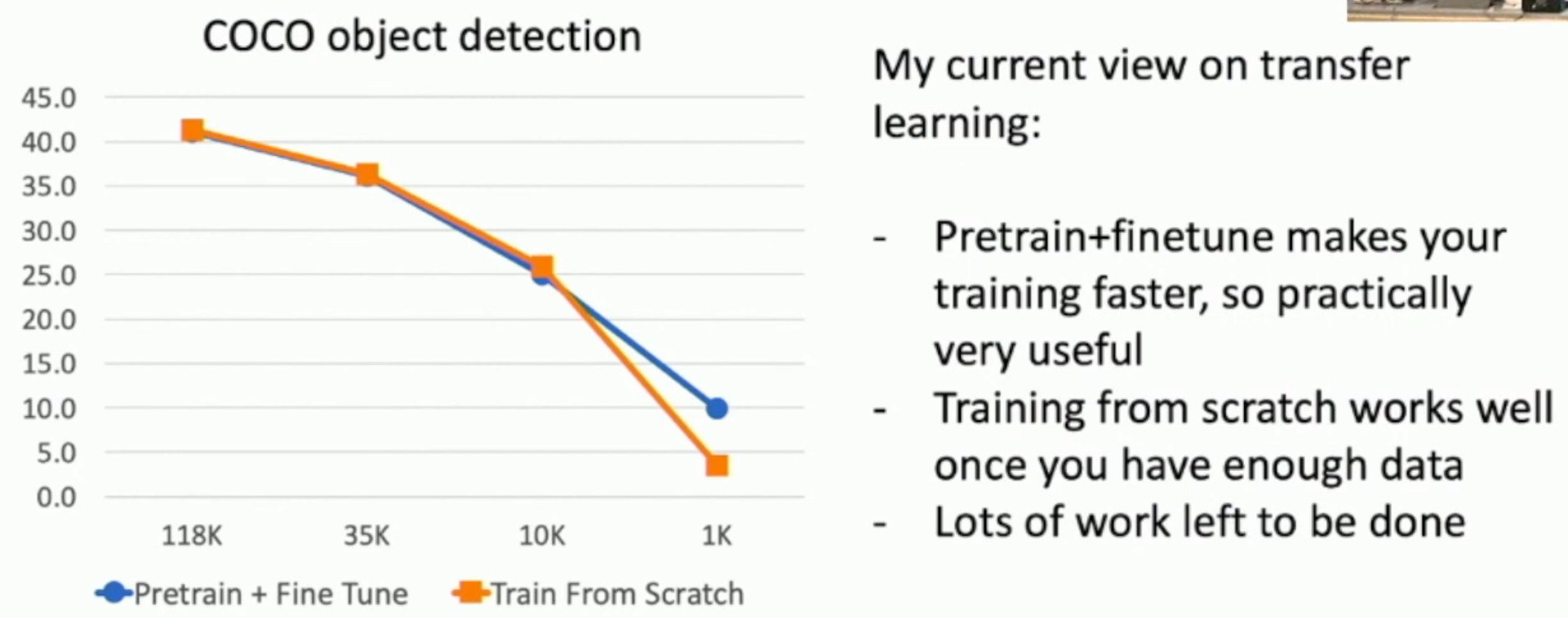
另外,对于较小样本的情况,pre-training + fine-tuning 的效果还是更好(右图)。
因此,我们可以得出几个规律
- Pretrain + fine-tuning 一般是不差于 traning from scratch 的
- 即使你的数据量很丰富,pretrain + fine-tuning 可以节省时间
Large-Batch Learning
In modern days,我们一般不会使用 model parallelism,而是使用 data parallelism,如下图所示:
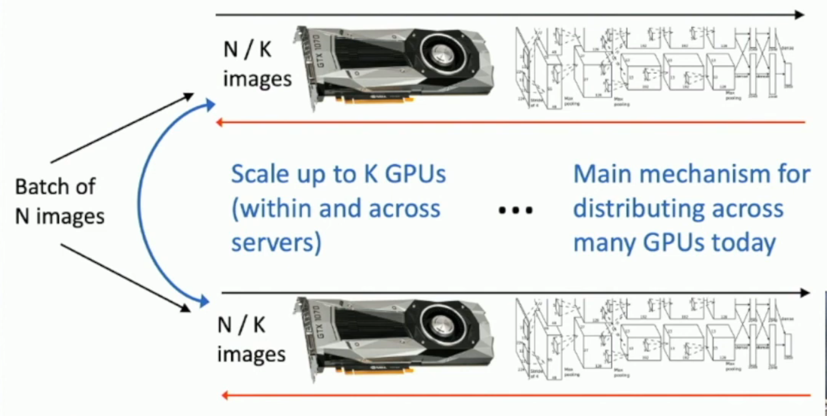
这是因为,model parallelism 往往要涉及到多个 GPU 之间的大量通信;而 data parallelism 会因为 batches 之间的独立性,而往往不太需要 GPU 之间的通信。
- 对于 data parallelism,我们唯一需要通信的地方,就是最后 aggregate the gradient