Error Analysis for Iterative Methods
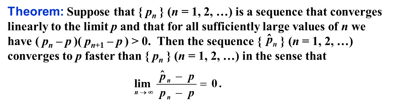
Definition: Suppose \(\set{p_n} (n=0,1,2,\dots)\) is a sequence that converges to \(p\), with \(p_n \neq p\) for all \(n\). If positive constants \(\alpha\) and \(\lambda\) exist with $$ \lim_{n\to\infty} \frac{\lvert p_{n+1} - p \rvert}{\lvert p_n - p \rvert^\alpha} = \lambda $$ then \(\set {p_n} (n=0,1,2,\dots)\) converges to \(p\) of order \(\alpha\), with asymptotic error constant \(\lambda\).
- If \(\alpha = 1\), the sequence is linearly convergent
- If \(\alpha = 2\), the sequence is quadratically convergent
Newton's Method: Revisited
Analysis of Convergence
牛顿法就是: $$ p_{n+1} = p_n - \frac {f(p_n)} {f'(p_n)} $$ 通过 Taylor's Method: $$ 0 = f(p) = f(p_n) + f'(p_n) (p - p_n) + \frac 1 2 f''(\xi_n)(p - p_n)^2 $$ 因此: $$ p = p_n - \frac {f(p_n)} {f'(p_n)} - \frac {f''(\xi_n)} {2! f'(p_n)} (p-p_n)^2 = p_{n+1} - \frac {f''(\xi_n)} {2! f'(p_n)} (p-p_n)^2 $$ 从而: $$ \frac{\lvert p_{n+1} - p \rvert}{\lvert p_n - p \rvert^2} = \frac {\frac {f''(\xi_n)} {2! f'(p_n)} (p-p_n)^2} {(p - p_n)^2} = \frac {f''(\xi_n)} {2 f'(p_n)} $$
- As long as \(f'(p) \neq 0\), Newton's method is AT LEAST quadratically convergent
NOTE:
- For general fixed point method, this doesn't hold - it can be as bad as linearly convergent.
- If the root is a simple root, it guarantees fast convergence locally, not globally. Thus you have to try multiple initial values (i.e. \(p_0\)) to get the correct answer, and also make sure the multiplicity of the root is 1.
Sidenote: How much time do I need with different α?
假设一次迭代的耗时为 \(t\),我们的期望精度为 \(eps\),初始误差为 \(e_0\)。
又假设 \(\frac{e_{n+1}}{e_n^\alpha} = \frac{\lvert p_{n+1} - p \rvert}{\lvert p_n - p \rvert^\alpha} \approx \lambda, \alpha > 1\),那么 $$ \ln e_{n+1} \approx \ln \lambda + \alpha \ln e_n \iff \ln e_{n+1} + \frac 1 {\alpha - 1} \ln \lambda \approx \alpha (\ln e_n + \frac 1 {\alpha - 1} \ln \lambda) $$ 从而: $$ \alpha^{\frac T t} (\ln e_n + \frac 1 {\alpha - 1} \ln \lambda) \approx \ln eps + \frac 1 {\alpha - 1} \ln \lambda $$ 也就是说: $$ T \approx \frac{\ln(-(\ln eps + \frac 1 {\alpha - 1} \ln \lambda)) - \ln(-(\ln e_n + \frac 1 {\alpha - 1} \ln \lambda))}{\ln \alpha} t = \mathcal O(\frac{\ln\ln eps} {\ln \alpha}t) $$
- 当然,如果 \(\alpha = 1\),那么 \(e_0 \lambda^{\frac T t} = eps \implies T = \frac{\ln eps - \ln e_0}{\ln \lambda}t\)
假如 \(\lambda_1 = 0.5, \lambda_2 = 0.8\),\(\alpha_1 = 1, \alpha_2 = 2\),\(e_n = 10^{-1}, eps = 10^{-10}, t = 1 \text{ hr}\),那么,
使用如下函数:
from math import *

def T_not_one(eps, a, l, e0, t):
    eps_ln = log(-(log(eps) + 1 / (a - 1) * log(l)))
    e0_ln = log(-(log(e0) + 1 / (a - 1) * log(l)))
    return (eps_ln - e0_ln) / log(a) * t


def T(eps, a, l, e0, t):
    if (a != 1):
            return T_not_one(eps, a, l, e0, t)
    else:
            return t * (log(eps) - log(e0)) / log(l)


l1, l2 = 0.9, 0.9
a1, a2 = 1, 2
e0 = 1e-1
eps = 1e-12
t = 1

T1, T2 = T(eps, a1, l1, e0, t), T(eps, a2, l2, e0, t)
day1, day2 = floor(T1 / 24), floor(T2 / 24)
hr1, hr2 = T1 - day1 * 24, T2 - day2 * 24

print(f"T1: {day1} days and {hr1:.1f} hours")
print(f"T2: {day2} days and {hr2:.1f} hours")
结果:
可见两者的差距很大。特别地,\(\alpha = 2\) 的时候,总用时对 \(\lambda, eps\) 其实并不太敏感(因为都是 \(\ln\ln\));而 \(\alpha = 1\) 的时候,对 \(eps\) 和 \(\lambda\) 其实很敏感。
Sidenote: General Practical Method for Determine α and λ
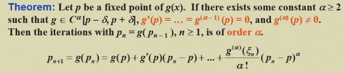
- 证明:由于 \(g(p) = p\),上式也就是:\(p_{n+1} - p = \frac {g^{\alpha}(\xi_n)} {\alpha !} (p_n - p) ^\alpha\),从而易证。
以牛顿法为例: $$ g(x) = x - \frac{f(x)}{f'(x)} $$ 因此: $$ \lim_{x\to x_0}g'(x) = \frac{f(x_0)f''(x_0)}{f'(x_0)^2} =0 \quad \text{ (as long as } f'(x_0) \neq 0) $$ 又因为: $$ g''(x) = \frac{f{\left(x \right)} \frac{d^{3}}{d x^{3}} f{\left(x \right)}}{\left(\frac{d}{d x} f{\left(x \right)}\right)^{2}} - \frac{2 f{\left(x \right)} \left(\frac{d^{2}}{d x^{2}} f{\left(x \right)}\right)^{2}}{\left(\frac{d}{d x} f{\left(x \right)}\right)^{3}} + \frac{\frac{d^{2}}{d x^{2}} f{\left(x \right)}}{\frac{d}{d x} f{\left(x \right)}} $$ 由于 \(f''(x_0)\) 一般并不为 0,所以 \(g''(x_0)\) 一般也不为 0,所以一般 \(\alpha = 2\)。和我们之前的结果一样。
Problem With Multiple Roots
对于 \(k\) 重根的情况: $$ f(x) = (x-x_0)^kq(x) \implies f'(x) = k(x-x_0)^{k-1} q(x) + (x-x_0)^{k}q'(x) \newline \implies f'(x_0) = \begin{cases} 0 \quad \text{if }k \geq 2 \newline q(x_0) \neq 0 \quad \text{if } k = 1 \end{cases} $$ 因此,对于多重根的情况,牛顿迭代法的性能会迅速下降。
- 具体地,如果有多重根,那么牛顿法的 \(\alpha = 1\),而且 \(\lambda = \frac{g'(p)}{1!} = 1 - \frac 1 k < 1\),因此虽然收敛,但是只是 1 阶收敛,而且随着 \(k\) 的增加,收敛时间会近似线性增加(i.e. \(-\frac 1 {\ln \lambda} = -\frac 1 {\ln (1 - \frac 1 k)} \approx k\))。
如何处理这样的问题呢?可以使用 modified version(如下)。
Modified Newton's Method
我们令 \(\mu(x) = \frac {f(x)} {f'(x)}\),从而 \(g(x) = x - \frac{\mu(x)}{\mu'(x)} = x - \frac{f(x)f'(x)}{[f'(x)]^2 -f(x)f''(x)}\)
如果 \(f(x) = (x-x_n)^kq(x)\),而且 \(q(x_n) \neq 0\)那么: $$ \mu(x) = \frac{(x-x_n)^kq(x)}{k(x-x_n)^{k-1}q(x) + (x-x_n)^{k}q'(x)} = \frac{(x-x_n)q(x)}{kq(x) + (x-x_n)q'(x)} \implies \newline \mu'(x) = \frac{[q(x) + (x-x_n)q'(x)][kq(x) + (x-x_n)q'(x)] - [(k+1)q'(x) + (x-x_n)q''(x)][(x-x_n)q(x)]}{\left[kq(x) + (x-x_n)q'(x)\right]^2} \implies \newline \mu'(x_n) = \frac{kq^2(x_n)}{k^2q^2(x_n)} = \frac{1}{k} $$ 从而,满足了 \(\mu'(x_0) \neq 0\) 的性质,使得迭代速率仍然可以为二阶。
Problems:
- 需要额外计算 \(f''(x)\)
- 由于 \([f'(x)]^2 -f(x)f''(x)\) 是两个很小的数相减,因此当两者接近的时候,relative rounding error 就会非常大。
Accelerating Methods
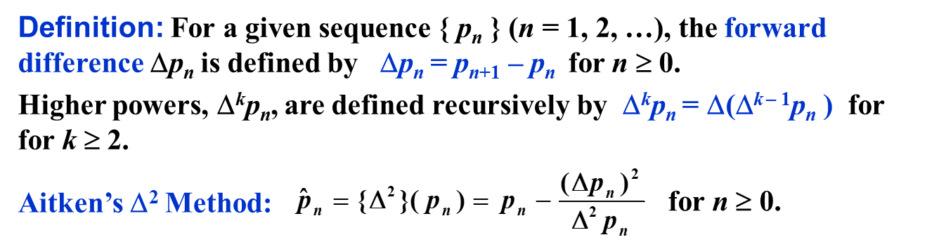
Aitken's Δ2 Method
Intuition
由于 $$ \frac { p _ { n + 1 } - p } { p _ { n } - p } \approx \lambda \newline \frac { p _ { n + 2 } - p } { p _ { n + 1 } - p } \approx \lambda $$ 因此,直觉上,两个式子应该也“差不多”。 $$ \begin{aligned} \frac { p _ { n + 1 } - p } { p _ { n } - p } &\approx \frac { p _ { n + 2 } - p } { p _ { n + 1 } - p } \newline
( p _ { n + 1 } - p ) ( p _ { n + 1 } - p ) &\approx ( p _ { n + 2 } - p ) ( p _ { n } - p ) \newline
p _ { n + 1 } ^ { 2 } - 2 p _ { n + 1 } p + p ^ { 2 } &\approx p _ { n + 2 } p _ { n } - ( p _ { n + 2 } + p _ { n } ) p + p ^ { 2 } \newline
- 2 p _ { n + 1 } p + ( p _ { n + 2 } + p _ { n } ) p &\approx p _ { n + 2 } p _ { n } - p _ { n + 1 } ^ { 2 } \newline
p &\approx \frac { p _ { n + 2 } p _ { n } - p _ { n + 1 } ^ { 2 } } { - 2 p _ { n + 1 } + ( p _ { n + 2 } + p _ { n } ) } \newline
p &\approx p _ { n } - \frac { ( p _ { n + 1 } - p _ { n } ) ^ { 2 } } { p _ { n + 2 } - 2 p _ { n + 1 } + p _ { n } } \end{aligned} $$ 从而,我们得到了一个关于 \(p\) 的 intuitive 的式子。我们不妨就直接用右边的式子代替 \(g(x)\): $$ \widehat p_n = p _ { n } - \frac { ( p _ { n + 1 } - p _ { n } ) ^ { 2 } } { p _ { n + 2 } - 2 p _ { n + 1 } + p _ { n } } $$
Definition
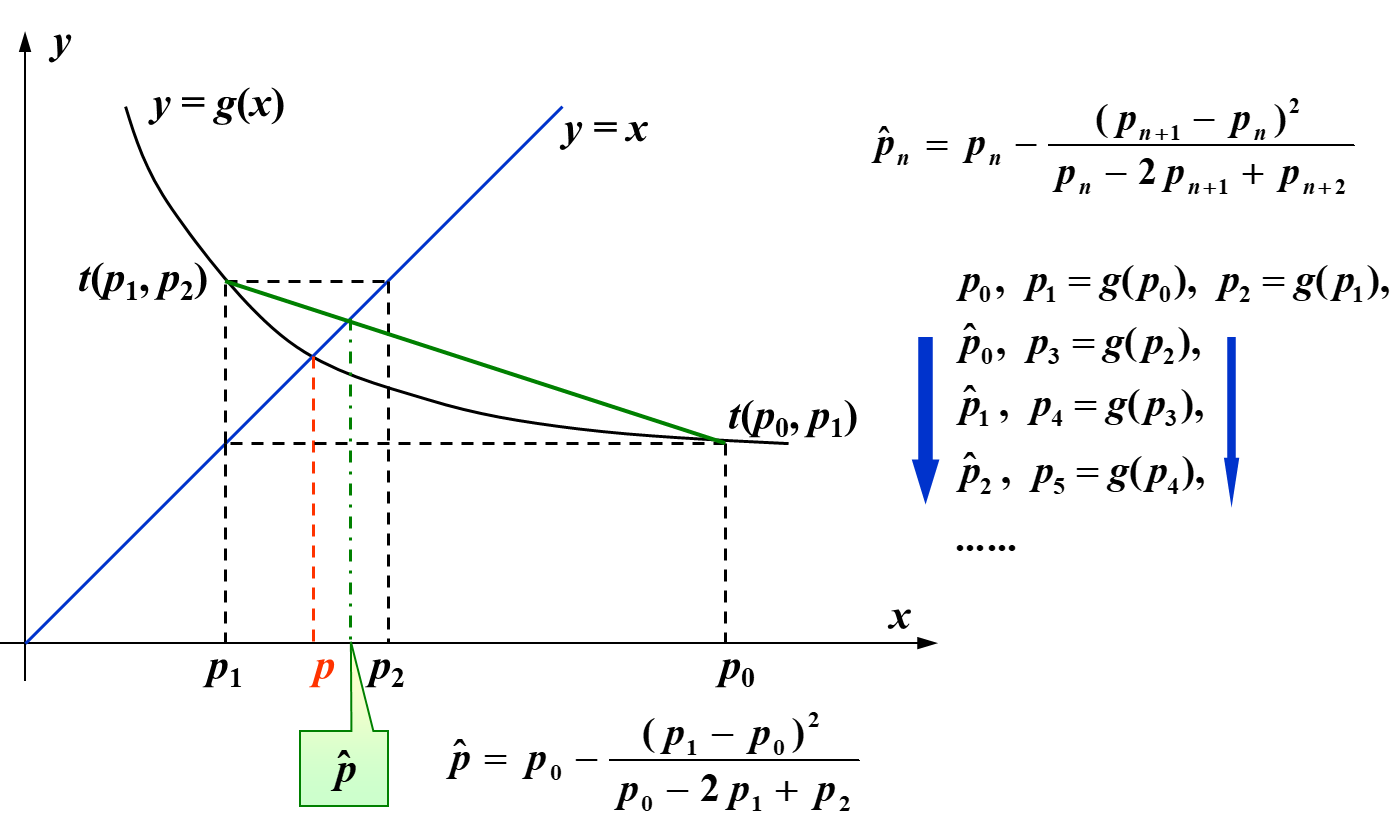
Calculation Steps
- 首先算出 \(\set{p_0, p_1, \dots}\)
- 然后通过 \(p_i, p_{i+1}, p_{i + 2}\) 算出 \(\widehat p_{i}\)
- 我们用 \(\widehat p_n\) 代替 \(p_n\) 作为最后的输出
下图就是形象的计算过程:
WARNING:
- 不可以认为 \(\widehat p_n\) 比 \(p_n\) “精确”,就自作聪明,在 \(\widehat p_n\) 算出来之后,再反过来通过它来计算 \(p_{n+1}, p_{n+2}, p_{n+3}\)(e.g. \(p_4 = g(g(g(\widehat p_1)))\),而非 \(p_4 = g(p_3)\))。因为 \(\widehat p_n\) 更加精确某种意义上来说,是“概率性”的、“不可预知”的,因此不能混用。
- 递归计算不能够无限优化,i.e. \(\set{\widehat {\widehat p}_n}, \set{\widehat {\widehat {\widehat p}}_n}, \dots\) 的收敛性并不会趋于无穷大。这就像多次压缩文件无法使其变成 1 byte 一样。
Analysis
Steffensen’s Method
虽然 Aitken's Δ2 Method 不可以混用,但是,不能混用的原因是混用可能会导致 \(\set{p_n}\) 不再是线性数列。
Aitken's Δ2 Method 最少需要 3 个数来计算出来 \(\widehat p_0\),因此,我们可以三个一组,每组均采用递推的方法计算(保证是线性数列),然后得到 \(\widehat p_0\),当作”新的起点“,然后再用 \(\widehat p_0\) 继续这样做,so on and so forth。
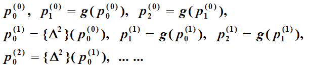
形象地看,如下图,序列整体不是线性的,但是每个方框内的小序列是线性的。箭头指的是用前一个方框的三个值,推出新的方框的第一个值。

由于方框内均为线性以及层层地推,由归纳法可知,所有方框均比上一个更优。
- 实际上,如果 \(g'(p) \neq 1\),则这样的迭代满足 local quadratic convergence。
Direct Method for Solving Linear Systems
定义:解形如 \(A\mathbf x=B\) 这样的线性方程组
Amount of Computation
由于
- 单个乘除计算的 cycle 较多
- 乘除对数值稳定性的破坏性较大
我们在分析线性系统的数值算法的时候,只考虑乘除运算的数量。
Example: Gaussian Elimination
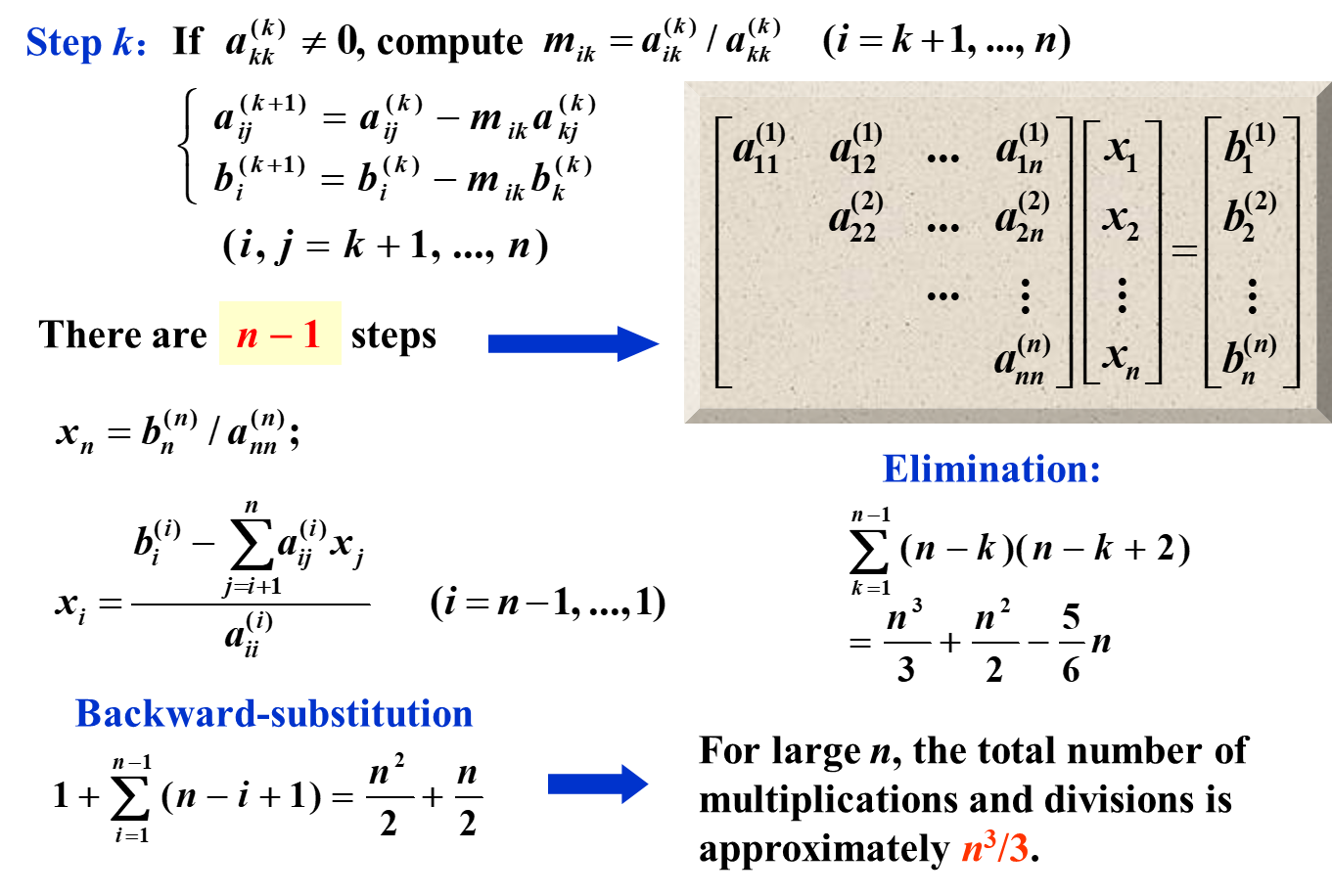
Naive 高斯消元的计算复杂度为 \(n^3\)。